Download
1 / 51
510 likes | 517 Views
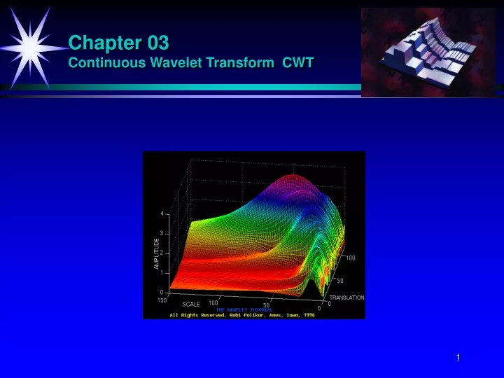
Chapter 03 Continuous Wavelet Transform CWT. Vectors in 2-dim R 2 Basis - Properties. 4. v. v. 1. e 2. e 2. e 1. 5. e 1. 2. Vectors in 2-dim R 2 Different basis. k 2 = 4e 1 + 6e 2. v. v. 2. k 1 = 2e 1 + e 2. e 2. e 1. 3. Inner product Examples. Vectors in R n.

E N D
Vectors in 2-dim R2Basis - Properties 4 v v 1 e2 e2 e1 5 e1 2
Vectors in 2-dim R2Different basis k2 = 4e1 + 6e2 v v 2 k1 = 2e1 + e2 e2 e1 3
Inner productExamples Vectors in Rn Vectors in C2 Polynomials ai C Continuous functions on the interval [a,b]
Hilbert-roomL2([a,b]) - Inner product f Sampling of f on the interval [a,b] = [0,1]: 0 1
Multiresolution Analysis (MRA) V0 V1 V2
Multiresolution V0 V1 V2 V3 V4 W0 W1 W2 W3
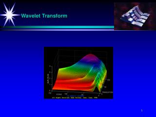
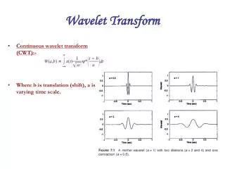
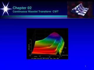
Definition of the CWT The continuous-time wavelet transform (CWT) of f(t) with respect to a wavelet (t):
Mother WaveletDilation / Translation Mother Wavelet s Dilation Scale Translation
Definition of a mother Wavelet (or Wavelet) A real or complex-value continuous-time function (t) satisfying the following properties, is called a Wavelet: 1. Wavelet 2. Finite energy 3. Admissibility condition. Sufficient, but not a necessary condition to obtain the inverse.
The Haar Wavelet and The Morlet Wavelet Haar Morlet 1 1 -1
Dilation / Translation: Haar Wavelet Haar 1 1 1 2-1/2 2-1/2 1 4 2 4 4 2 -1 -1 -1
Mexican Hat Mexican Hat
Forward / Inverse Transform Forward Inverse Mother Wavelet s Dilation Scale Translation
Admissibility condition It can be shown that square integrable functions (t) satisfying the admissibility condition can be used to first analyze and then reconstruct a signal without loss of information. Admissibility condition. Sufficient, but not a necessary condition to obtain the inverse. The admissibility condition implies that the Fourier transform of (t) vanishes at the zero frequency. Wavelets must have a band-pass like spectrum. A zero at the zero frequency also means that the average value of the wavelet in the time domain must be zero. (t) must be oscillatory, it must be a wave.
Regularity conditions - Vanishing moments The time-bandwidth product of the wavelet transform is the square of the input signal. For most practical applications this is not a desirable property. Therefor one imposes some additional conditions on the wavelet functions in order to make the wavelet transform decrease quickly with decreasing scale s. These are the regularity conditions and they state that the wavelet function should have some smoothness and concentration in both time and frequency domains. Taylor series at t = 0 until order n (let = 0 for simplicity): pth moment of the wavelet Moments up to Mn is zero implies that the coefficients of W(s,t) will decay as fast as sn+2 for a smooth signal. Oscillation + fast decay = Wave + let = Wavelet
Multi-scale differential operator [1/2] Estimating the regularity of a signal is closely linked to the concept of vanishing moments. Definition: A function has k vanishing moments when Wavelets vanishing moments are linked to the so-called smoothing functions. Definition: A function is a smoothing function if its integral is equal to 1 and it converges to 0 at infinity. If is a smoothing function, then so is a(t) = a-1/2 (k)(t), and large a correspond to heavy smoothing.
Multi-scale differential operator [2/2] Wf(a,b) smooth or low-pass filters f on a frequency interval proportional to a and then differentiates k times. We have a description of f(k) across scales.
CWT - Correlation 1 Cross- correlation CWT CWT W(s,) is the cross-correlation at lag (shift) between f(t) and the wavelet dilated to scale factor s.
CWT - Correlation 2 W(a,b) always exists The global maximum of |W(a,b)| occurs if there is a pair of values (a,b) for which ab(t) = f(t). Even if this equality does not exists, the global maximum of the real part of W2(a,b) provides a measure of the fit between f(t) and the corresponding ab(t) (se next page).
CWT - Correlation 3 The global maximum of the real part of W2(a,b) provides a measure of the fit between f(t) and the corresponding ab(t) ab(t) closest to f(t) for that value of pair (a,b) for which Re[W(a,b)] is a maximum. -ab(t) closest to f(t) for that value of pair (a,b) for which Re[W(a,b)] is a minimum.
CWT - Localization both in time and frequency The CWT offers time and frequency selectivity; that is, it is able to localize events both in time and in frequency. Time: The segment of f(t) that influences the value of W(a,b) for any (a,b) is that stretch of f(t) that coinsides with the interval over which ab(t) has the bulk of its energy. This windowing effect results in the time selectivity of the CWT. Frequency: The frequency selectivity of the CWT is explained using its interpretation as a collection of linear, time-invariant filters with impulse responses that are dilations of the mother wavelet reflected about the time axis (se next page).
CWT - Frequency - Filter interpretation Convolution CWT CWT is the output of a filter with impulse response *ab(-b) and input f(b). We have a continuum of filters parameterized by the scale factor a.
CWT - Time and frequency localization 1 Time Center of mother wavelet Frequency Center of the Fourier transform of mother wavelet
CWT - Time and frequency localization 2 Time Frequency Time-bandwidth product is a constant
CWT - Time and frequency localization 3 Time Frequency Small a: CWT resolve events closely spaced in time. Large a: CWT resolve events closely spaced in frequency. CWT provides better frequency resolution in the lower end of the frequency spectrum. Wavelet tool a natural tool in the analysis of signals in which rapidly varying high-frequency components are superimposed on slowly varying low-frequency components (seismic signals, music compositions, …).
CWT - Time and frequency localization 4 a=1/2 a=1 a=2 t Time-frequency cells for a,b(t) shown for varied a and fixed b.
Basis-functions for Hilbert room L2(0,2).Fourier transformation. Fourier-serie Ortonormale basis-funksjoner Dilation Generering
Basis-functions Hilbert room L2(R).Wavelet transformation. Wavelet-serie Ortonormale basis-funksjoner Dilation, translation Generering
TeoremProof Use the following notation:
TeoremProof Use the following notation:
Binary dilation / Dyadic translation Binary dilation Dyadic translation
Filtering / Compression Data compression Remove low W-values Highpass-filtering Lowpass-filtering Replace W-values by 0 for high a-values Replace W-values by 0 for low a-values
Inverse Wavelet transformation 1 WT Dual IWT = WT-1 Modifisert
Inverse Wavelet transformation 2 a,b R WT Condition Basic Wavelet Inverse Dual
Inverse Wavelet transformation 3 a,b Ra > 0 WT Condition Inverse Dual
Inverse Wavelet transformation 4 a,b Ra = 1/2j WT Condition Dyadic Wavelet Inverse Dual
Basic Wavelet Def L2(R) kalles en basic wavelet hvis følgende betingelse er oppfylt: Herav navnet wavelet
Wavelet-Based Edge Detectionin Ultrasound Images [2/5] The wavelet scale dependent spectrum is a measure of the distribution of energy of the signal f(t) as a function of scale. The energy of the signal. The spectrum S divided by the square of the scale is the energy contribution for that scale, while the square of the wavelet coefficients represents the local energy content.
Wavelet-Based Edge Detectionin Ultrasound Images [3/5] Detection:
SINTEF Unimed, Ultrasound [1/2] - For simple cases the range of scales around the optimal will find the egde - For more complex images, this may not be the case, and it is of crucial importance to find the correct scale. - Noise may shift the scale. - False detection are made at beams in which two or more occurrences of structure of approximately the same size and intensity are found. - No false detection because of small-scale high intensity noise. - What about the angle between beam and membrane? - Estimate the scale from several beams, using the value that occurs most often. - Use of filter to remove high frequency noise. - Other wavelets (Daubechies, …)
SINTEF Unimed, Ultrasound [1/2] - CWT (Forward / Inverse) Noise - Filtering - Thresholding - Multiple beams - Gradients - First max …
DNRDetection of Microcalcifications in Mammograms - Preprocessing: - Statistical differencing - Gaussian filtering - Signal extraction and background suppresssion: - CWT - Area and amplitude thresholding: - Global thresholding - Area limitations - Local maxima extaction - Local thresholding - Shape analysis - Gradient measurements - Karhunen-Loeve analysis - Wavelet analysis: - Amplitude across scales - Correlation and clustering - Clusteres microcalcifications