Download
1 / 58
580 likes | 583 Views
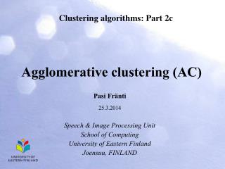
Fast Agglomerative Clustering for Rendering. Bruce Walter, Kavita Bala, Cornell University Milind Kulkarni, Keshav Pingali University of Texas, Austin. P. Q. R. S. Clustering Tree. Hierarchical data representation Each node represents all elements in its subtree

E N D
Fast Agglomerative Clustering for Rendering Bruce Walter, Kavita Bala, Cornell University Milind Kulkarni, Keshav Pingali University of Texas, Austin
P Q R S Clustering Tree • Hierarchical data representation • Each node represents all elements in its subtree • Enables fast queries on large data • Tree quality = average query cost • Examples • Bounding Volume Hierarchy (BVH) for ray casting • Light tree for Lightcuts
Tree Building Strategies • Agglomerative (bottom-up) • Start with leaves and aggregate • Divisive (top-down) • Start root and subdivide P Q R S
Tree Building Strategies • Agglomerative (bottom-up) • Start with leaves and aggregate • Divisive (top-down) • Start root and subdivide P Q R S
Tree Building Strategies • Agglomerative (bottom-up) • Start with leaves and aggregate • Divisive (top-down) • Start root and subdivide P Q R S
P Q R S Tree Building Strategies • Agglomerative (bottom-up) • Start with leaves and aggregate • Divisive (top-down) • Start root and subdivide
P Q R S Tree Building Strategies • Agglomerative (bottom-up) • Start with leaves and aggregate • Divisive (top-down) • Start root and subdivide
P Q R S Tree Building Strategies • Agglomerative (bottom-up) • Start with leaves and aggregate • Divisive (top-down) • Start root and subdivide
P Q R S Tree Building Strategies • Agglomerative (bottom-up) • Start with leaves and aggregate • Divisive (top-down) • Start root and subdivide P Q
P Q R S P Q R S Tree Building Strategies • Agglomerative (bottom-up) • Start with leaves and aggregate • Divisive (top-down) • Start root and subdivide
Conventional Wisdom • Agglomerative (bottom-up) • Best quality and most flexible • Slow to build - O(N2) or worse? • Divisive (top-down) • Good quality • Fast to build
Goal: Evaluate Agglomerative • Is the build time prohibitively slow? • No, can be almost as fast as divisive • Much better than O(N2) using two new algorithms • Is the tree quality superior to divisive? • Often yes, equal to 35% better in our tests
Related Work • Agglomerative clustering • Used in many different fields including data mining, compression, and bioinformatics [eg, Olson 95, Guha et al. 95, Eisen et al. 98, Jain et al. 99, Berkhin 02] • Bounding Volume Hierarchies (BVH) • [eg, Goldsmith and Salmon 87, Wald et al. 07] • Lightcuts • [eg, Walter et al. 05, Walter et al. 06, Miksik 07, Akerlund et al. 07, Herzog et al. 08]
Overview • How to implement agglomerative clustering • Naive O(N3) algorithm • Heap-based algorithm • Locally-ordered algorithm • Evaluating agglomerative clustering • Bounding volume hierarchies • Lightcuts • Conclusion
Agglomerative Basics • Inputs • N elements • Dissimilarity function, d(A,B) • Definitions • A cluster is a set of elements • Active cluster is one that is not yet part of a larger cluster • Greedy Algorithm • Combine two most similar active clusters and repeat
Dissimilarity Function • d(A,B): pairs of clusters -> real number • Measures “cost” of combining two clusters • Assumed symmetric but otherwise arbitrary • Simple examples: • Maximum distance between elements in A+B • Volume of convex hull of A+B • Distance between centroids of A and B
Naive O(N3) Algorithm Repeat { Evaluate all possible active cluster pairs <A,B> Select one with smallest d(A,B) value Create new cluster C = A+B } until only one active cluster left • Simple to write but very inefficient!
Naive O(N3) Algorithm Example U T P Q S R
Naive O(N3) Algorithm Example U T P Q S R
Naive O(N3) Algorithm Example U T P Q S R
Naive O(N3) Algorithm Example U T PQ S R
Naive O(N3) Algorithm Example U T PQ S R
Naive O(N3) Algorithm Example U T PQ S R
Naive O(N3) Algorithm Example U T PQ RS
Acceleration Structures • KD-Tree • Finds best match for a cluster in sub-linear time • Is itself a cluster tree • Heap • Stores best match for each cluster • Enables reuse of partial results across iterations • Lazily updated for better performance
Heap-based Algorithm Initialize KD-Tree with elements Initialize heap with best match for each element Repeat { Remove best pair <A,B> from heap If A and B are active clusters { Create new cluster C = A+B Update KD-Tree, removing A and B and inserting C Use KD-Tree to find best match for C and insert into heap } else if A is active cluster { Use KD-Tree to find best match for A and insert into heap } } until only one active cluster left
Heap-based Algorithm Example U T P Q S R
Heap-based Algorithm Example U T P Q S R
Heap-based Algorithm Example U T P Q S R
Heap-based Algorithm Example U T PQ S R
Heap-based Algorithm Example U T PQ S R
Heap-based Algorithm Example U T PQ S R
Heap-based Algorithm Example U T PQ RS
3 3 1 2 1 2 P P Q Q R R S S Locally-ordered Insight • Can build the exactly same tree in different order • How can we use this insight? • If d(A,B) is non-decreasing, meaning d(A,B) <= d(A,B+C) • And A and B are each others best match • Greedy algorithm must cluster A and B eventually • So cluster them together immediately =
Locally-ordered Algorithm Initialize KD-Tree with elements Select an element A and find its best match B using KD-Tree Repeat { Let C = best match for B using KD-Tree If d(A,B) == d(B,C) { //usually means A==C Create new cluster D = A+B Update KD-Tree, removing A and B and inserting D Let A = D and B = best match for D using KD-Tree } else { Let A = B and B = C } } until only one active cluster left
Locally-ordered Algorithm Example U T P Q S R
Locally-ordered Algorithm Example U T P Q S R
Locally-ordered Algorithm Example U T P Q S R
Locally-ordered Algorithm Example U T P Q S R
Locally-ordered Algorithm Example U T P Q S R
Locally-ordered Algorithm Example U T P Q RS
Locally-ordered Algorithm Example U T P Q RS
Locally-ordered Algorithm Example U T P Q RS
Locally-ordered Algorithm Example U T P Q RS
Locally-ordered Algorithm Example U T P Q RS
Locally-ordered Algorithm Example U T PQ RS
Locally-ordered Algorithm • Roughly 2x faster than heap-based algorithm • Eliminates heap • Better memory locality • Easier to parallelize • But d(A,B) must be non-decreasing
Results: BVH • BVH – Binary tree of axis-aligned bounding boxes • Divisive [from Wald 07] • Evaluate 16 candidate splits along longest axis per step • Surface area heuristic used to select best one • Agglomerative • d(A,B) = surface area of bounding box of A+B • Used Java 1.6JVM on 3GHz Core2 with 4 cores • No SIMD optimizations, packets tracing, etc.
Results: BVH Kitchen Temple Tableau GCT
Results: BVH Surface area heuristic with triangle cost = 1 and box cost = 0.5