Download
1 / 75
820 likes | 1.05k Views
Isoquants, Isocosts and Cost Minimization Overheads. We define the production function as. y represents output. f represents the relationship between y and x. x j is the quantity used of the jth input. (x 1 , x 2 , x 3 , . . . x n ) is the input bundle.

E N D
We define the production function as y represents output f represents the relationship between y and x xj is the quantity used of the jth input (x1, x2, x3, . . . xn) is the input bundle n is the number of inputs used by the firm
y Holding other inputs fixed, the production function looks like this y = f (x1, x2, x3, . . . xn ) 350 300 Output-y 250 200 150 100 50 0 0 2 4 6 8 10 12 Input -x
Marginal physical product Marginal physical product is defined as the increment in production that occurs when an additional unit of a particular input is employed
A MPP Graphically marginal product looks like this 60 50 Output -y 40 30 20 10 0 1 2 3 4 5 6 7 8 9 10 11 -10 -20 -30 -40 Input -x
The Cost Minimization Problem Pick y; observe w1, w2, etc; choose the least cost x’s
Isoquants An isoquant curve in two dimensions represents all combinations of two inputs that produce the same quantity of output The word “iso”means same while “quant” stand for quantity
Isoquants are contour lines of the production function If we plot in x1 - x2 space all combinations of x1 and x2 that lead to the same (level) height for the production function, we get contour lines similar to those you see on a contour map Isoquants are analogous to indifference curves Indifference curves represent combinations of goods that yield the same utility Isoquants represent combinations of inputs that yield the same level of production
There are many ways to produce 2,000 bales of hay per hour Workers Tractor-Wagons Total Cost AC 10 1 80 0.04 6.45 1.66 71.94 .03597 5.48 2 72.8658 0.0364 3.667 3 82.0015 0.041 2.636 4 95.8167 0.0479 1.9786 5 111.872 .0559
Isoquant y = 2000 x2 = 4, x1 = 2.636 Or Isoquant y = 2,000 12 X 10 1 8 6 4 2 0 0 2 4 6 8 10 12 14 X 2
Only the negatively sloped portions of the isoquant are efficient
Isoquant for y = 10,000 x1 x2 output y -- 1 10,000 -- 2 10,000 -- 3 10,000 12.469 4 10,000 9.725 5 10,000 8.063 6 10,000 6.883 7 10,000 5.990 8 10,000 5.290 9 10,000
Isoquant y = 2000 Isoquant y = 10000 Graphical representation Isoquants y = 2,000, y = 10,000 14 12 x1 10 8 6 4 2 0 0 2 4 6 8 10 12 14 x 2
Slope of isoquants An increase in one input (factor) requires a decrease in the other input to keep total production unchanged Therefore, isoquants slope down (have a negative slope)
Properties of Isoquants Higher isoquants represent greater levels of production Isoquants are convex to the origin This means that as we use more and more of an input, its marginal value in terms of the substituting for the other input becomes less and less
Slope of isoquants The slope of an isoquant is called the marginal rate of (technical) substitution [ MR(T)S ] between input 1 and input 2 The MRS tells us the decrease in the quantity of input 1 (x1) that is needed to accompany a one unit increase in the quantity of input 2 (x2), in order to keep the production the same
Isoquant y = 2000 Isoquant y = 10000 The Marginal Rate of Substitution (MRTS) 14 12 x1 10 8 6 4 2 0 0 2 4 6 8 10 12 14 x 2
Algebraic formula for the MRS The marginal rate of (technical) substitution of input 1 for input 2 is We use the symbol - | y = constant - to remind us that the measurement is along a constant production isoquant
Example calculations y = 2,000 Workers Tractor-Wagons x1 x2 10 1 5.48 2 3.667 3 2.636 4 1.9786 5 Change x2 from 1 to 2
Example calculations y = 2,000 Change x2 from 2 to 3 Workers Tractor-Wagons x1 x2 10 1 5.48 2 3.667 3 2.636 4 1.9786 5
More example calculations y = 10,000 x1 x2 12.469 4 9.725 5 8.063 6 6.883 7 5.990 8 Change x2 from 5 to 6
A declining marginal rate of substitution The marginal rate of substitution becomes larger in absolute value as we have more of an input. The amount of an input we can to give up and keep production the same is greater, when we already have a lot of it. When the firm is using 10 units of x1, it can give up 4.52 units with an increase of only 1 unit of input 2, and keep production the same But when the firm is using only 5.48 units of x1, it can only give up 1.813 units with a one unit increase in input 2 and keep production the same
Slope of isoquants and marginal physical product Marginal physical product is defined as the increment in production that occurs when an additional unit of a particular input is employed
Marginal physical product and isoquants All points on an isoquant are associated with the same amount of production Hence the loss in production associated with x1 must equal the gain in production from x2 , as we increase the level of x2 and decrease the level of x1
Rearrange this expression by subtracting MPPx2 x2 from both sides, Then divide both sides by MPPx1 Then divide both sides by x2
The left hand side of this expression is the marginal rate of substitution of x1 for x2, so we can write So the slope of an isoquant is equal to the negative of the ratio of the marginal physical products of the two inputs at a given point
The isoquant becomes flatter as we move to the right, as we use more x2 (and its MPP declines) and we use less x1 ( and its MPP increases) So not only is the slope negative, but the isoquant is convex to the origin
Isoquant y = 2000 The Marginal Rate of Substitution (MRTS) 14 12 x1 10 8 6 4 2 0 0 2 4 6 8 10 12 14 x 2
Approx x1 x2 MRS MPP1 MPP2 12.4687 4.0000 --- 664.6851 2585.7400 11.8528 4.1713 -3.5946 739.5588 2465.2134 9.7255 5.0000 -2.5672 1010.5290 2050.0940 9.3428 5.1972 -1.9411 1063.1321 1975.4051 8.0629 6.0000 -1.5941 1254.9695 1724.5840 6.9792 6.9063 -1.1959 1447.3307 1508.9951 6.8827 7.0000 -1.0291 1466.3867 1489.5380
Approx x1 x2 MRS MPP1 MPP2 12.4687 4.0000 --- 664.6851 2585.7400 11.8528 4.1713 -3.5946 739.5588 2465.2134 9.7255 5.0000 -2.5672 1010.5290 2050.0940 9.3428 5.1972 -1.9411 1063.1321 1975.4051 8.0629 6.0000 -1.5941 1254.9695 1724.5840 6.9792 6.9063 -1.1959 1447.3307 1508.9951 6.8827 7.0000 -1.0291 1466.3867 1489.5380 x2 rises and MRS falls
Isocost lines An isocost line identifies which combinations of inputs the firm can afford to buy with a given expenditure or cost (C), at given input prices. Quantities of inputs - x1, x2, x3, . . . Prices of inputs - w1, w2, w3, . . .
Graphical representation Cost = 120 w1 = 6 w2 = 20 22 20 x 1 18 16 14 12 10 8 6 4 2 0 0 1 2 3 4 5 6 7 x 2
Slope of the isocost line So the slope is -w2 / w1