Download
1 / 99
1.11k likes | 1.67k Views
Cost Minimization. Accountants vs. Economists. Economists think of costs differently from accountants. Economics Cost = Explicit Costs + Implicit Costs Accounting Cost = Explicit Costs Opportunity Cost is synonymous with Cost Measuring implicit opportunity costs is difficult

E N D
Accountants vs. Economists • Economists think of costs differently from accountants. • Economics Cost = Explicit Costs + Implicit Costs • Accounting Cost = Explicit Costs • Opportunity Cost is synonymous with Cost • Measuring implicit opportunity costs is difficult • generally, these are resources “owned” by the firm • Includes the value of the entrepreneur’s time • Includes accounting profit at next best alternative use of firm’s resources – or, accounting profit from selling all owned resources and investing the proceeds in the best possible alternative investment.
Fixed Cost and Sunk Cost • Fixed vs. Sunk cost • “fixed” means its cost does not vary with output • “sunk” means its cost cannot be avoided • The security guard outside the parking lot is a fixed cost, but if they can be fired at a moment’s notice, the cost is not sunk • A long term lease for renting a building is fixed and sunk • Varian calls a fixed cost that is not sunk a “quasi-fixed cost” • Sunk, but not fixed? No, because if it varies, it can be avoided.
Short Run – Long Run • Key distinction in terms of optimizing behavior if everything can be controlled vs. not everything can be controlled. • Short run, the quantities of some inputs used in production are fixed and some are variable. • Short run, firms can shut down (q=0), but cannot exit the industry • Long run, the quantity of all inputs used are variable. • Long run, firms can enter or exit an industry.
To Distinguish Short Run from Long Run • We need two inputs, one always variable, and one that can only be adjusted periodically, but is then re-fixed. • To accomplish that, we assume two inputs • Homogeneous labor (L), measured in labor per time • Homogeneous capital (K), measured in machine per time • Entrepreneurial costs assumed to be zero (or included in fixed costs) • Inputs are hired in perfectly competitive markets, so price of L, w, and price of K, v, are not a function of L and K
To be clear • L is assumed always variable • K is always fixed when the firm is in production, but can periodically be adjusted to a new fixed amount (so in the long run it can be varied to a new fixed amount). • That is, production always takes place in a short run situation.
Notation • K, capital; v, rental rate of capital • L, Labor; w, wage rate
Cost • Clearly, C can be stated as: C = vK + wL • But this is meaningless, we need cost as a function of output, not K and L. • To get that, back to the production function
Graphically q q3 q2 K q1 q = f(K, L) q0 An entire range of input combinations can be used to produce every level of output. q3 q2 q1 q0 L
Short Run, K constant q = f(K=K3, L) q q = f(K=K2, L) q = f(K=K1, L) q3 q2 Possible to produce the same level of output at different combinations of K and L. q1 L Three different slices through the production function at different levels of K.
Short Run, K constant Let’s look at just one slice. q q2 At some fixed level of K, for every q, we know how much L it will take. L2 L
Production to Cost Flip the axis L q q L
Production to Cost L L = L(q,K) q
Production to Cost SC = w·L(q)+vK Multiply L by w to get labor cost $/time VC = w· L(q) Add in FC, SC=SVC+FC FC q
Production to Cost SC = w· L(q)+rK And we can figure a few things $/time VC = w· L(q) FC q
Production to Cost SAC $ SMC AVC AFC q
Short Run, K constant q = f(K=K3, L) q q = f(K=K2, L) Inflection point, q3 q = f(K=K1, L) Inflection point, q2 With more K, you can produce more with a given L and the inflection point moves towards more L and q. Inflection point, q1 L What does that mean for cost curves?
Production to Cost $ SC = w· L2(q)+rK2 SC = w· L3(q)+rK3 Inflection Points SC = w· L1(q)+rK1 FC q Fixed cost is higher with more K, but the inflection point is further to the right, with a slower build-up of crowding.
C C $ SC = w· L2(q)+rK2 SC = w· L3(q)+rK3 SC = w· L1(q)+rK1 q C is the lowest point on any of the SC curves for any q
SAC $ Min value at higher q with more K. SAC = C2/q SAC = C1/q SAC = C3/q LAC q AC is the lowest point on any of the SR ATC curves for any q
MC C $ MC is the slope of the C curve at any q q
Short Run – Long Run • Firms ALWAYS produce in a short run situation with at least one fixed and one variable input. • Being in the long run simply means the firm has adjusted to an optimal level of capital to minimize the cost of producing any chosen (profit maximizing) level of output.
Different Shapes for the long run C Curve C $ There are four different potential shapes q
C -- CRS C $ CRS, as K and L are scaled upwards, C rises at the same rate. That is, MC is constant. q
C -- CRS $ Min value at higher q with more K. ATC = TC2/q ATC = TC1/q ATC = TC3/q AC=MC q CRS, as K and L are scaled upwards, LAC rises at the same rate. That is, LAC is constant.
C -- IRS C $ IRS, as K and L are scaled upwards, C rises more slowly That is, MC is decreasing. q
C -- IRS $ AC MC q CRS, as K and L are scaled upwards, AC rises at a slower rate. AC is decreasing.
C -- DRS $ DRS, as K and L are scaled upwards, TC rises faster That is, MC is increasing. C q
LTC -- DRS Note, it is not the low point of each ATC curve, but the simply the lowest point on any ATC. $ MC AC q CRS, as K and L are scaled upwards, AC rises at a faster rate. AC is increasing.
C – IRS, CRS, DRS C $ IRS, then CRS, then DRS q
C – IRS, CRS, DRS So we have a U-shaped AC curve for a completely different reason than the SAC curve is U-shaped. $ MC AC q
Firm Decisions • So which short run curve should we be on? • That is, how much K (and then L) do we want to hire (with K fixed in the SR)? • Two choices • Profit Maximization: Firms maximize profit by choosing q*, K and L to minimize cost all at once. • Cost minimization: Firms choose a q*, then choose K and L to minimize the cost of producing q*.
Profit Maximization • Economic profits () are equal to = total revenue - total cost • Total costs for the firm are given by C = wL + vK • Total revenue for the firm is given by total revenue = R = p·q = p·f(K,L) • Economic profits () are equal to = p·f(K,L) - wL - vK
Profit Maximization • Solving to maximize profit means jointly choosing q = q* along with K* and L*. • Yields profit maximizing factor (input) demand functions which provide L* and K* that minimizes the cost of producing q*. • When r, w, and p change, L*, K*, and q* all change. • L*=L(w, v, p); K*=K(w, v, p); q*=q(w, v, p) • These functions allow for a change in q* (the isoquant) when prices change.
Cost Minimization • That firms minimize cost is a weaker hypothesis of firm behavior than profit maximization. • Yields quantity constant (quantity contingent) factor (input) demand functions which provide L* and K* that minimize the cost of producing q0. • When r and w change, L* and K* do change, but q does not, stay on one isoquant. • Why bother? It is how we get the cost functions and curves (i.e. what we use in principles and intermediate micro)
New Direction in Graphing • In all the graphs above, we have illustrated the long run as a series of short run curves and traced out the envelope. • Good for intuition, but not terribly tied to the math of the optimization • Let’s switch to the isoquant graph.
Intuitively Isoquant, all combinations of factors that yield the same output. Slope is -dK/dL K Isocost (total cost), all combinations of factors that yield the same total cost of production. Slope is -w/v L
Cost-Minimizing Input Choices • When K and L change a small amount • Along an Isoquant,
Cost-Minimizing Input Choices • TRS is the change in K needed to replace one L while maintaining output. • Minimum cost occurs where the TRS is equal to w/v • the rate at which Kcan be traded for L in the production process = the rate at which they can be traded in the marketplace
Intuitively w=20, v=10 w/v=2 • Firing one L has MB of $20 and MC of $2.5 • Lowers cost by $17.50 K TRS=.25 L
Intuitively w=20, v=10 w/v=2 • Firing one L has MB of $20 and MC of $10 • Lowers cost by $10 K TRS=1 L
Intuitively w=20, v=10 w/v=2 • Firing one L has MB of $20 and MC of $15 • Lowers cost by $5 K TRS=1.5 L
Intuitively w=20, v=10 w/v=2 • Firing one L has MB of $20 and MC of $20 • Lowers cost by $0 • Further reductions in L require an increase in cost as TRS >w/r. K TRS=2 L
Intuitively w=20, v=10 w/v=2 • Firing one L has MB of $20 and MC of $25 • Raises cost by $5 K TRS=2.5 L
Plan • Figure out the quantity of K and L that minimize total cost, holding q constant. • Use the resulting factor demand curves to derive the cost functions.
Cost-Minimizing Input Choices • We seek to minimize total costs given q =q0 q = f(K,L) = q0 • Setting up the Lagrangian: FOCs are
Cost-Minimizing Input Choices • Dividing the first two conditions we get • The cost-minimizing firm should equate the RTS for the two inputs to the ratio of their prices • But also • Which tells us that for the last unit of all inputs hired should provide the same bang-for-the-buck.
Cost-Minimizing Input Choices • The inverse of this equation is also of interest • The value of the Lagrange multiplier is the extra costs that would be incurred by increasing the output constraint slightly by hiring enough L or K to increase output by 1. • That is λ = MC of increasing production by one unit.
Cost-Minimizing Input Choices • SOC to ensure costs are RISING, along the isoquant, away from the tangency: • Bordered Hessian The part in brackets is the same condition required for strict quasi concavity of the production function
Intuitively w=20, r=10 w/r = 2 • Cost minimized for q0 when L=L* and K=K * K SOC satisfied as moving along the isoquant means increasing TC Total Cost RTS=2 K* L* L