Download
1 / 38
390 likes | 566 Views
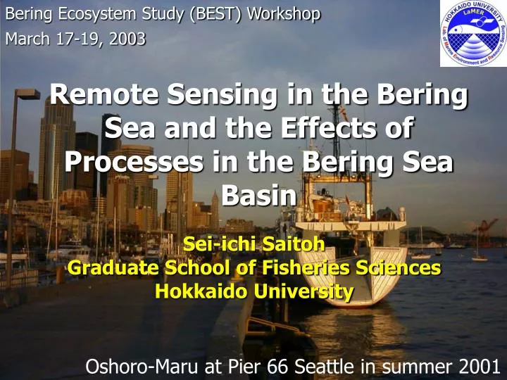
Bering Ecosystem Study (BEST) Workshop. March 17-19, 2003. Remote Sensing in the Bering Sea and the Effects of Processes in the Bering Sea Basin. Sei-ichi Saitoh Graduate School of Fisheries Sciences Hokkaido University. Oshoro-Maru at Pier 66 Seattle in summer 2001. Contents. Background

E N D
Bering Ecosystem Study (BEST) Workshop March 17-19, 2003 Remote Sensing in the Bering Sea and the Effects of Processes in the Bering Sea Basin Sei-ichi Saitoh Graduate School of Fisheries Sciences Hokkaido University Oshoro-Maru at Pier 66 Seattle in summer 2001
Contents • Background • Two Topics • - Coccolithophore Bloom dynamics during 1997-2002 • - Seasonal and interanual variability of Bering Sea Eddies along the green belt • Future Application • Some Suggestions
Background OCEAN DEPTHS OF THE ARCTIC OCEAN AND ADJACENT SEAS Max Depth 5450 m Ecosystem Studies of Sub-Arctic Seas Program
Study Area Arctic Ocean North-South Linkage Okhotsk Sea Bering Sea West-East Comparison
The Green Belt (Springer et al., 1996) Coccolitophore Blooming Ship Observation (1995-2002) Sediment Trap (1990-2002) Bering Sea Eddies
Two Topics Bering Sea Ecosystem from Space • Coccolithophore Bloom dynamics during 1997-2002 • Seasonal and interanual variability of Bering Sea Eddies along the green belt
Two Topics Bering Sea Ecosystem from Space • Coccolithophore Bloom dynamics during 1997-2002 • Seasonal and interanual variability of Bering Sea Eddies along the green belt
・OCTS Coccolithophore mask image in 1997 spring SeaWiFS coccolithophore bloom Image from Sep.19 to Oct.3 nLw(443)>1.1 nLw(565)>0.8 0.64<nLw(443/565)<1.55 0.7<nLw(443/520)<1.0 0.93<nLw(520/565)<1.6 May 1997 OCTS Coccolithophore mask Image Iida et al. (2002) →OCTS found 1997 bloom!!
・ Variability of coccolithophore bloom and Sea Ice Coccolithophore bloom area Composite Monthly Sea ice and Coccolithophore Mask Image
・ Variability of coccolithophore bloom and Sea Ice Coccolithophore bloom area Composite Monthly Sea ice and Coccolithophore Mask Image
・ 5 years Variability of coccolithophore bloom area ・1998 →massive summer bloom ・1999 →weak spring and fall bloom ・2000 →massive bloom(Apr.Jun.Sep.) ・2001 →low sea ice concentration weak bloom ・2002 →weak bloom
・ SST anomaly and coccolithophore blooms Pixel number Histogram of SST anomaly in cocco bloom area 1998 Summer July 1998 SST anomaly Image Positive SST Anomaly!!
・ SST anomaly and coccolithophore blooms Pixel number Histogram of SST anomaly in cocco bloom area 1999 Summer August 1999 SST anomaly Image Negative SST Anomaly!!
Conclusions • Coccolithophore Blooms • We found coccolithophore bloom using OCTS image in spring, before observation by SeaWiFS image in autumn 1997. • Coccolithophore bloom of Emiliania huxleyi began spring and distributed at the surface layer from 20m to 100m in depth in the southeastern Bering Sea Shelf. • Large bloom in 1998 and 2000, weak bloom in 1999 2001 and 2002. Positive sea surface temperature(SST) anomaly was corresponding to occurrence of massive coccolithophore blooms, and might triggered increasing coccolithophore biomass in 1998 and 2000 summer.
Two Topics Bering Sea Ecosystem from Space • Coccolithophore Bloom dynamics during 1997-2002 • Seasonal and interanual variability of Bering Sea Eddies along the green belt
4892-78 Background mg/m3 1. Shelf-Slope exchange Stabeno et al., 1999 2. Nutrient supply & high chl-a concentration Sapozhnikov, V.V., 1993 Mizobata et al., 2002 3. Positive correlation of Walleye pollock larvae & Bering Sea eddies Schumacher and Stabeno, 1994 Napp et al., 2000 4. High Iron & Low Nutrient of Shelf water Low Iron & High Nutrient of Basin water McRoy et al., 2001 May-Jun 2001
Questions Little are known about the horizontal distribution of mesoscale eddies along the shelf edge…. How many eddies are there along the shelf edge? How much impacts does it affect on phytoplankton distribution and primary production along the ”Green Belt”?
Data and Method 1. TOPEX/ERS-2daily Sea Surface Height Anomaly (SSHA) image 1998 Jan.1. ~ 2001 Dec.30 ( http://www-ccar.colorado.edu/research/topex/html/topex.html) 2. TOPEX/Poseidon 10days cycle SSHA 1997 Jan. ~ 2001 Dec (cycle 158 ~ 342) 3. Orbview2/SeaWiFS L3 chl-a concentration 1997 October. ~ 2001 May 4. Primary production calculated from SeaWiFS chl-a, PAR and NOAA/ AVHRR sea surface temperature using Kameda and Ishizaka model [advanced VGPM model] 1997 October. ~ 2001 May
30days 244(H:124, L:120) in 1998 256(H:137, L:119) in 1999 312(H:141, L:171) in 2000 324(H:150, L:174) in 2001 Results - 1 : Lifetime of eddies
Zhemchug canyon Pribilof canyon Results - 2 : Bering Sea eddy field 10 days cycle data along the shelf break of the Bering Sea D-79 SSHAs calculated from Merged Geophysical Data Record – B[JPL] (Benada,1997)
0.43cm/s(1998) 0.54cm/s(1999) 1.0~1.8cm/s(2000-2001) A Results - 2 : Bering Sea eddy field B 01/11/02 Time-latitude isopleths of T/P SSHAs
About 6months High PPeu Low PPeu Results - 3 : Biological conditions(PPeu) No data Time-latitude isopleths of primary production estimated using Kameda and Ishizaka model(2002)
Results - 3 : Biological conditions(PPeu) Averaged primary production along the shelf break
Conclusions Bering Sea eddies and primary production Satellite Remote sensing revealed, • The interannual variability of Bering Sea eddy • field affected by the BSC transport. • (From 2000, there was an increase in Bering Sea • eddy field.) • 2. Difference in Propagation and distribution • characteristics between cyclonic and anti- • cyclonic eddy • 3. An importance of Bering Sea eddy field for • maintaining the productivity.
Future Application Bering Sea Ecosystem from Space New method of sea ice thickness estimation using passive microwave radiometers Tateyama et al. (2002) - amount of sea ice production interannual - variability of sea ice thickness New ocean color data sets and Multi-sensor SeaWiFS, two MODISs (from Aqua and Terra) and GLI (from ADEOS-II) The frequency of shutter chances is increasing and hyper-spectral data sets are available.
N=108 R=0.81 ó=14cm New method of sea ice thickness estimation H(cm) = -537.33・PR + 83.88・R37V/85V – 6.91 Tateyama et al. (2002)
Inter-seasonal out-of-phase response in the Okhotsk Sea and the Bering Sea Okhotsk > Bering Okhotsk < Bering Tateyama et al. (2002)
New method of sea ice thickness estimation Accumulated ice volume Tateyama et al. (2003), unpublished
New ocean color data sets and Multi-sensor Chlorophyll a August 2002 MODIS Suspended Matter August 2002 MODIS
New ocean color data sets and Multi-sensor April 7, 2002 MODIS False Color image
New ocean color data sets and Multi-sensor ADEOS-II SeaWinds (Microwave) Four days composite(Jan. 28- Jan. 31, 2003)
Some Suggestions • Bio-optical drifting buoy(TOGA-TAO type) to study time-series primary production and biogeochemical process • ARGO-type bio-optical buoy system (such as K-SOLO) to study vertical structure of biological processes in the basin region of the Bering Sea
Ed Lu Some suggestions: Instrumentation Ed, AT, Ba Bio-optical Drifting Buoy Sensors 1.Barometer (Ba) 2.Sea Surface Temperature(SST) 3.Air Temperature(AT) 4.Lu(683nm) 5.Lu(670nm) 6.Lu(555nm) 7.Lu(510nm) 8.Lu(490nm) 9.Lu(443nm) 10.Lu(412nm) 11.Ed(490nm) 1m Lu, SST
Chl=0.59807*(Lu443/Lu555)-1.04598 Chl=0.56353*(Lu443/Lu555)-0.595 Abbott,1995 Some suggestions: Instrumentation Bio-optical Drifting Buoy 15Station TSRB R2=0.80 TSRB Obs. map Mooring optical buoy
2001/8/07 2001/8/17 2001/7/27 Comparison trajectory with TOPEX and SeaWiFS data 2001 8/17 8/07 7/27
Anti-cyclonic Spin out Cyclonic Variability of SST and chl-a field in 2001 8/17 Chl SST 8/07 7/27
Some suggestions: Instrumentation Bio-optical Drifting Buoy Alaska 9/20 8/10 12/18 10/18 3/3 Aleutian Arc 1/11 Buoy Track Aug.2002-Mar.2003
Thank you Photo by Sei-ichi Saitoh Baby Island, Aleutian Islands in Summer, 1975