Download
1 / 24
250 likes | 386 Views
Information Science 2 -Random Numbers and Monte Carlo Method-. College of Information Science and Engineering Ritsumeikan University. Autumn : Week 13. Terms and concepts from Week 12 The concept of random variables Simple descriptive statistics Probability density and mass functions

E N D
InformationScience 2-Random Numbers andMonte Carlo Method- College of Information Science and EngineeringRitsumeikan University Autumn : Week 13
Terms and concepts from Week 12 • The concept of random variables • Simple descriptive statistics • Probability density and mass functions • Mathematical expectation • Variance • Random and pseudorandom numbers and their generation • Monte Carlo simulation • Test Agenda
Random experiment • Uncertainty, Variability • Sample space, Simple events • Probability • Complement • Mutual exclusivity • Conditional probability • Bayes' Theorem • Independent and dependent events Recall concepts from Week 12
Learn the concepts of random variables and random numbers • Overview the Monte Carlo method and its applications • After this lecture and study, you must be able to: • Understand the concepts of and work with random variables and random numbers • Understand the idea of Monte Carlo simulation This lecture’s objective
Random variables • A random variable is the outcome of a random experiment represented in a numerical form • A random variable can, therefore, be seen as a function that maps the sample space of a random experiment to (a subset of) R or Z • A random variable is discrete if the number of the experiment’s possible outcomes is finite or countable • Discrete random variables are evaluated by count (e.g. Web-site visits, traffic accidents, etc.) • A random variable is continuous if the experiment’s possible outcomes cannot completely be listed but can take on any value within an interval • Continuous random variables are evaluated through measurement (e.g. temperature, weight, etc.)
Descriptive statistics • Suppose we conduct a random experiment – measure the air temperature in two different classrooms for 10 days. The outcome of this experiment will be some 20 values • What are the chances that the temperature is +25ºC in either of the two rooms on the next day after we finished the experiment?Based solely on our observations,which room is likely to be colder? • To answer such questions, we use descriptive statistics – functions that represent the main properties of a collection of data in a quantitative form
Probability density function • For a continuous random variable, the basic descriptive statistics are determined with a probability density function (PDF) that describes the relative likelihood for the random variable to take on a specific value in the sample space • Let f(x) be a PDF of the continuous random variable X measured in our “room temperature” experiment. Based on f(x), we can estimate the chances that the temperature in either of the rooms is within a given interval (a, b](e.g.24.99ºC < temperature 25ºC) using the following formula:
PDF and Histogram • In many cases, the specific form of f(x), the PDF can be determined from a relevant theory • For example, for temperature, a Gamma PDF is often used, which has the following shape: • When we have no appropriate theory but only experimental measurements ofX, a histogram can be used to estimate f(x) • A histogram shows what proportion of data falls into each of several predefined intervals
The case of discrete variables • The discrete analog of a PDF is a probability mass function (PMF) that gives the probability that a discrete random variable is exactly equal to a specified value • All values of a PMF must be non-negative numbers that sum up to 1 • A histogram is used “as is” to estimate fX (x), the PMF of a discrete random variable X • The height of each bar corresponds to the probability of the particular value of X • When the width of the bar is 1, the area of each bar corresponds to the probability that the value x will occur • Descriptive statistics are often easier to compute in the case of discrete random variables
Basic descriptive statistics • The (mathematical) expectation (also called the expected value or mean) E(X) of a discrete random variable X can be estimated as: • The varianceVar(X) of a discrete random variable X can be estimated as: • Here, xi are the specific (measured) values of the discrete random variable X, N the number of xi
Expectation and variance • The expectation of a random variable tells us the average (but not the most probable!) value of that random variable(e.g. it may be 23.05ºC in the first room, and 24.3ºC in the second – the second room is then said to be warmer on average) • The variance 2of a random variable is a measure of the amount of variation within the values of that variable • In practice, the standard deviation , which is the square root of the variance, is often used and gives a measure of the data variability – the “spread” of the corresponding PMF or PDF
Random numbers • In engineering and science, instead of computing descriptive statistics based on empirical (i.e. measured) data, we also often have to model a random variable (i.e. generate its values), using a particular PDF f(x) from theory • Two types of numbers can be used to model outcomes of a random experiment: • True random numbers (TRN) – numbers that are not predictable and not repeatable in principle • Pseudorandom numbers (PRN) – numbers that appear random, but are obtained with deterministic, repeatable, and predictable methods
True random numbers • To generate true random numbers, various non-deterministic sources of randomness can be used: • Decay times of radioactive material • Thermal or electrical noise from a resistor or semiconductor • Radio channel or audible noise, etc. • Methods of true random number generation are usually slow and require special (expensive) hardware
Pseudorandom numbers • Computers are deterministic and thus cannot be used to generate true random numbers • However, computers can generate pseudorandom numbers • The first machine used to produce a table of 100,000 random digits was done byM. G. Kendall and B. Babington-Smith in 1939 • RAND Corporation in 1955 released a table of a million random digits generated with a computer • Function RND() is supported by nearly all modern programming languages
PRN generation: A simple algorithm • For uniformly-distributed PRN generation, a Linear Congruential Generator (LCG) can be used as follows:int RND(){seed = seed*A+B;return (unsigned int)(seed/(N*2))%N;} • The variable seed is a global variable that can be set before beginning the sequence • A, B, and N are integer constants:N is the range of pseudorandom integers we want; A and B make a computation large enough to emulate randomness after mod N
PRN generation: Algorithm evaluation criteria • A PRN generation algorithm can be evaluated by the following four criteria: • Produces sequences of (equiprobable) values with a uniform distribution • Each specific output cannot be predicted • There is no repetition for short sequences • A sequence can be repeated using the same seed • The RND() function on the previous slide satisfies these criteria sufficiently for many applications • This function, however, may not be “good enough” for secure applications, such as encryption
Monte Carlo methods • A major application of pseudorandom numbers is Monte Carlo methods (also called Monte Carlo simulation) • Monte Carlo methods use random numbers and descriptive statistics to model problems • Key components of Monte-Carlo simulation: • Probability distribution function (PDF): required to describe the system to be analyzed • Random number generator • Sampling rule: to obtain the required PDF from uniform PRNs • Tallying (or scoring): to calculate averaged results
10cm Monte Carlo simulation: An example • Estimate the area of a circle drawn in a square withside = 10cm, using Monte Carlo Method • Theoretically, the area of a circle is A=PI*r*r, so A=PI*5*5, or about 78.5 cm2 • The accuracy of the answer depends on how accurate the value for the constant PIis • With Monte Carlo simulation, we can hit the square with random points and see how many points “fall on” the circle
Monte Carlo simulation: An example (cont-d) • The simulation algorithm: • Determine a suitable PDF (uniform in this case; in principle, however, any PDF can be computed from a uniform PDF) • Simulate: Perform random sampling from the PDF, using the RND()function • Keep a record of each simulation performed and tally the counts
History of the Monte Carlo method • “Monte Carlo” comes from the gambling town of the same name in Europe • In science, Monte Carlo simulation was first used in 1947 to model diffusion of neutrons through fissile materials (to make a bomb) • Until recently, its application was limited because the simulation can require a lot of time to achieve reasonably precise results • Typical applications of Monte Carlo methods include DNA analysis, computing PI, and modeling human behavior
Simulation vs. Theoretical analysis • One of the major benefits of simulation is that it can be easy to set up • Another advantage is that low-level details (in our example, the shape of the geometrical object whose area is computed) may be easier to include than in theoretical analysis • A disadvantage, however, is that even a small error in the algorithm will lead to a completely wrong result • Another disadvantage is that it may be hard to find the “correct” theoretical PDF for simulation (when simulated events are not equiprobable)
Summary of this lecture After this class, you are expected to know the following: • What is a random variable • What are the basic descriptive statistics, and how are they used • The difference between random and pseudorandom numbers • The criteria to evaluate a PRN generation algorithm • What is Monte Carlo simulation
Homework • Read these Power Point slides • Do the self-preparation assignments • Learn the English terms new for you
Next class • Finite state automata and Turing machines • Alphabets, words, languages, and grammars • State diagrams • Finite state automation • The concept of Turing Machine