Download
1 / 21
220 likes | 425 Views
Hit-and-Miss (or Rejection) Monte Carlo Method: a “brute-force” method based on completely random sampling. y. Then, how do we throw the stones and count them on computer?. 1. A. (x i ,y i ). 1. Generation of M 2D microstates. x. O. 2. Measurement (Averaging an observable over

E N D
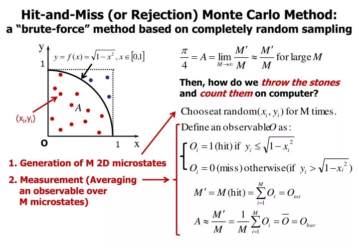
Hit-and-Miss (or Rejection) Monte Carlo Method: a “brute-force” method based on completely random sampling y Then, how do we throw the stones and count them on computer? 1 A (xi,yi) 1. Generation of M 2D microstates x O 2. Measurement (Averaging an observable over M microstates) 1
Lab 1. Calculation of the value of /4 Simple, Brute-Force, Hit-and-Miss Monte Carlo Method • Obtain an approximate value of A (= /4 M/M) by • throwing M stones in the square of the total area 1; • counting M stones in a quarter of the circle of the radius 1. • Question 1 (Formulation of the problem = Restatement of the last page). • On computer, this problem can be formulated as obtaining the average (or expectation value) of an observable O over M instantaneous Oi values at each microstate (xi, yi) (i = 1 to M). • What values can Oi take? • (2) How does the value of Oi depend on (xi, yi)?
Lab 1. Calculation of the value of /4 Simple, Brute-Force, Hit-and-Miss Monte Carlo Method • Obtain an approximate value of A (= /4 M/M) by • throwing M stones in the square of the total area 1; • counting M stones in a quarter of the circle of the radius 1. • Question 1 (Formulation of the problem = Restatement of the last page). • On computer, this problem can be formulated as obtaining the average (or expectation value) of an observable O over M instantaneous Oi values at each microstate (xi, yi) (i = 1 to M). • What values can Oi take? • Answer: 0 or 1 • (2) How does the value of Oi depend on (xi, yi)? • Answer:
Lab 1. Calculation of the value of /4 (or ) Question 2 (Algorithm & Flow chart). Draw a flow chart to estimate A (or = 4A) by averaging over M instantaneous Oi values.
Lab 1. Calculation of the value of /4 Otot = 0.0 Question 2 (Algorithm & Flow chart). Draw a flow chart to estimate A (or = 4A) by averaging over M instantaneous Oi values. Answer. i = 1 O = 0.0 x=ran3(&seed) y=ran3(&seed) yes no O = 1.0 Otot = Otot + O i = i + 1 no yes Obar = Otot/M; = 4xObar
Lab 1. Calculation of the value of /4 (or ) Question 3. Write a program to estimate A by averaging over M instantaneous O values. Try M = 10,000.
Otot = 0; input seed Flow chart for Question 4: Calculate . i = 1 O = 0.0 x=ran3(&seed); y=ran3(&seed) yes no O = 1.0 Otot = Otot + O i = i + 1 no yes Obar = Otot/M; = 4Obar; true = acos(-1); = fabs(true )
Lab 1. Calculation of the value of /4 (or ) Question 3. Write a program to estimate A by averaging over M instantaneous O values. Try M = 10,000.
Lab 1. Calculation of the value of /4 (or ) Question 6. But, what if we don’t know the true value of what we estimate? Since we can’t estimate the error w.r.t. the true value, how could we estimate the accuracy (error) of the simulation?
Lab 1. Calculation of the value of /4 (or ) Variance, Standard Deviation, Error, and Accuracy
Lab 1. Calculation of the value of /4 (or ) Variance, Standard Deviation, Error, and Accuracy
Otot = 0; O2tot =0; input seed Flow chart for Question 7: Calculate . i = 1 O = 0.0 x=ran3(&seed); y=ran3(&seed) yes O = 1.0 no Otot = Otot + O; O2tot = O2tot + O2 i = i + 1 no yes Obar = Otot/M; O2bar = O2tot/M; = sqrt(O2bar Obar2) pi = 4 x Obar; _pi = 4 x
Lab 1. Calculation of the value of /4 (or ) Answer: We expected that would be similar to ( ), but it’s not the case ( > ). (~constant with M) is much larger than (which decreases as M increases)! Thus, itself is not a good indicator of the accuracy of a simulation. Question 8. Then, what else would be an indicator of the accuracy (error) of the estimation, when we don’t know the true value of what we estimate?
Otot = 0; O2tot =0 Flow chart for Question 9: Calculate over n estimates. i = 1 O = 0.0 x=ran3(&seed); y=ran3(&seed) yes O = 1.0 one_estimate no Otot = Otot + O; O2tot = O2tot + O2 i = i + 1 no yes Obar = Otot/M; O2bar = O2tot/M; = sqrt(O2bar Obar2) pi = 4 x Obar; _pi = 4 x
Obartot= 0; Obarsqtot=0; tot = 0; input seed Flow chart for Question 9: Calculate over n estimates. j = 1 one_estimate Obartot = Obartot + Obar Obarsqtot = Obarsqtot + Obar2 tot = tot+ j = j + 1 no yes Obarbar = Obartot/n Obarsqbar = Obarsqtot/n bar= sqrt(Obarsqbar Obarbar2) bar= tot/n pi = 4xObarbar; barpi= 4xbar; barpi= 4xbar
Lab 1. Calculation of the value of /4 (or ) Question 10. But, what if we move onto a very complex problem? Each estimation (simulation) with M trials becomes so time-consuming that we couldn’t afford to running the simulation many times. What should we do in this case? Answer: Let’s try to find a way to estimate the accuracy from one M-trial simulation.