Download
1 / 49
580 likes | 765 Views
Room BI 115 Lecture: Monday, Wednesday Friday 2-3pm. Ch121a Atomic Level Simulations of Materials and Molecules. Lecture 5b and 61 , April 14 and 16, 2014 MD2: dynamics. William A. Goddard III, wag@wag.caltech.edu

E N D
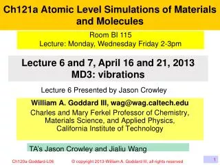
Room BI 115 Lecture: Monday, Wednesday Friday 2-3pm Ch121a Atomic Level Simulations of Materials and Molecules Lecture 5b and 61, April 14 and 16, 2014 MD2: dynamics William A. Goddard III, wag@wag.caltech.edu Charles and Mary Ferkel Professor of Chemistry, Materials Science, and Applied Physics, California Institute of Technology TA’s Jason Crowley and Jialiu Wang
Homework and Research Project First 5 weeks: The homework each week uses generally available computer software implementing the basic methods on applications aimed at exposing the students to understanding how to use atomistic simulations to solve problems. Each calculation requires making decisions on the specific approaches and parameters relevant and how to analyze the results. Midterm: each student submits proposal for a project using the methods of Ch121a to solve a research problem that can be completed in the final 5 weeks. The homework for the last 5weeks is to turn in a one page report on progress with the project The final is a research report describing the calculations and conclusions
Previously we develop the force fields and we minimized the geometry now we do dynamics
Classical mechanics – Newton’s equations Newton’s equations are Mk (d2Rk/dt2)= Fk = - RkE where Rk, Fk, and are 3D vectors and where goes over every particle k Here Fk = Sn≠kFnk where Fnk is the force acting on k due to particle n From Newton’s 3rd law Fnk = - Fkn Solving Newton’s equations as a function time gives a trajectory with the positions and velocities of all atoms Assuming the system is ergotic, we can calculate the properties using the appropriate thermodynamic average over the coordinates and momenta.
Consider 1D – the Verlet algorithm Newton’s Equation in 1D is M(d2x/dt2)t = Ft = - (dE/dx)t We will solve this numerically for some time step d. First we consider how velocity is related to distance v(t+d/2) = [x(t+d) – x(t)]/d; that is the velocity at point t+d/2 is the difference in position at t+d and at t divided by the time increment d. Also v(t-d/2) = [x(t) – x(t-d)]/d Next consider how acceleration is related to velocities a(t) = [v(t+d/2) - v(t-d/2)]/d = that is the acceleration at point t is the difference in velocity at t+d/2 and at t-d/2 divided by the time increment d. Now combine to get a(t)=F(t)/M= {[x(t+d) – x(t)]/d] - [x(t) – x(t-d)]/d)}/d = {{[x(t+d) – 2x(t) + x(t-d)]}/d2 Thus x(t+d) = 2x(t) - x(t-d) + d2 F(t)/M This is called the Verlet (pronounced verlay) algorithm, the error is proportional to d4. At each time t we calculate F(t) and combine with the previous x(t-d) to predict the next x(t+d)
Initial condition for the Verlet algorithm The Verlet algorithm, x(t+d) = 2x(t) - x(t-d) + d2 F(t)/M starts with x(t) and x(t-d) and uses the forces at t to predict x(t+d) and all subsequent positions. But typically the initial conditions are x(0) and v(0) and then we calculate F(0) so we need to do something special for the first point. Here we can write, v(d/2) = v(0) + ½ d a(0) and then x(d) = x(0) + d v(d/2) = x(0) + v(0) + ½ d F(0)/M As the special form for getting x(d) Then we can use the Verlet algorithm for all subsequent points.
Consider 1D – the Leap Frog Verlet algorithm Since we need both velocities and coordinates to calculate the various properties, I prefer an alternative formulation of the numerical dynamics. Here we write v(t+d/2) = v(t-d/2) +d a(t) and x(t+d) = x(t) + v(t+d/2) This is called leapfrog because the velocities leap over positions and the positions leap over the velocities Here also there is a problem at the first point where we have v(0) not v(d/2). Here we write v(0) = {v(d/2) + v(-d/2)]/2 and v(d/2) - v(-d/2) = d a(0) So that 2v(d/2) = d a(0) + 2 v(0) or v(d/2) = v(0) + ½ d F(0)/M
Usually we start with a structure, maybe a minimized geometry, but where do we get velocities? For an ideal gas the distribution of velocities follows the Maxwell-Boltzmann distribution, For N particles at temperature T, this leads to an average kinetic energy of KE= Sk=1,3N (Mk vk2/2)=(3N)(kBT/2) where kBis Boltzmann’s constant. In fact our systems will be far from ideal gases, but it is convenient to start with this distribution. Thus we pick a distribution of random numbers {a1,…,a3N} that has a Gaussian distribution and write vi =aisqrt[(2kT/M) This will lead to KE ~ (3N/2)(kBT), but usually we want to start the initial KE to be exactly the target bath TB. Thus we scale all velocities by l such that KE = (3N/2)(kBTB)
Equilibration Although our simulation system may be far from an ideal gas, most dense systems will equilibrate rapidly, say 50 picoseconds, so our choice of Maxwell-Boltzmann velocities will not bias our result Often we may start the MD with a minimized structure. If so some programs allow you to start with double Tbath. The reason is that for a harmonic system in equilibrium the Virial theorem states that <PE>=<KE>. Thus if we start with <PE>=0 and the KE corresponding to some Tinitial, the final temperature, after equilibration will be T ~½ Tinitial.
The next 4 slides are background material The Virial Theorem - 1 For a system of N particles, the Virial (a scalar) is defined as G = Sk (pk ∙ rk) where p and r are vectors and we take the dot or inner product. Then dG/dt = Sk (pk ∙ drk/dt) + Sk (dpk/dt ∙ rk) = Sk Mk(drk/dt ∙ drk/dt) + Sk (Fk ∙ rk) = 2 KE + Sk (Fk ∙ rk) Where we used Newton’s equation: Fk = dpk/dt Here Fk = Sn’Fnk is the sum over all forces from the other atoms acting on k, and the prime on the sum indicates that n≠k
The Virial Theorem - 2 Thus Sk (Fk ∙ rk) = Sk Sn’ (Fn,k ∙ rk) = Sk Sn<k (Fn,k ∙ rk) + Sk Sn>k (Fn,k ∙ rk) = Sk Sn<k (Fn,k ∙ rk) + Sk Sk>n (Fk,n ∙ rn) = Sk Sn<k (Fn,k ∙ rk) + Sk Sk>n (-Fn,k ∙ rk) = Sk Sn<k [Fn,k ∙ (rk – rn)] Where line 3 relabeled k,n in 2nd term and line 4 used Newton’s 3rd law Fk,n = - Fn,k . But Fn,k = - rk PE = - [d(PE)dr] [(rk – rn)/rnk] Sk (Fk ∙ rk) = - Sk Sn<k [d(PE)dr] [(rk – rn)]2/rnk = - Sk Sn<k [d(PE)dr] rnk
The Virial Theorem - 3 Using Sk (Fk ∙ rk) = - Sk Sn<k [d(PE)dr] rnk we get dG/dt = 2 KE - Sk Sn<k [d(PE)dr] rnk Now consider a system in which the PE between any 2 particles has the power law form, PE(rnk) = a (rnk)p for example: p=2 for a harmonic system and p=-1 for a Coulomb system. Then dG/dt = 2KE – p PEtot which applies to every time t. Averaging over time we get <dG/dt> = 2<KE> – p <PEtot>
The Virial Theorem - 4 <dG/dt> = 2<KE> – p <PEtot> Integrating over time ʃ0t (dG/dt) dt = G(t) - G(0) For a stable bound system G(∞)=G(0) Hence <dG/dt> = 0, leading to the Virial Theorem 2<KE> = p <PEtot> Thus for a harmonic system <KE> = <PEtot> = ½ Etotal And for a Coulomb system <KE> = -1/2 <PEtot> So that Etotal = ½ <PEtot> = - <KE>
microcanonical Dynamics (NVE) Solving Newton’s equations for N particles in some fixed volume, V, with no external forces, leads to conservation of energy, E. This is referred to as microcanonical Dynamics (since the energy is fixed) and denoted as (NVE). Since no external forces are acting on this system, there is no heat bath to define the temperature.
canonical Dynamics (NVT) – isokinetic energy • We will generally be interested in systems in contact with a heat bath at Temperature TB. In this case the states of the system should have (q,p) such that P(p,q) = exp[-H(p,q)/kBTB]/Z is the probability of the system having coordinates p,q. This is called a canonical distributions of states. • However, though we started with • KE= Sk=1,3N (Mk vk2/2)=(3N/2)(kBTB) there is no guarantee that the KE will correspond to this TB at a later time. • A simple fix to this is velocity scaling, where all velocities are scaled by a factor, l, such that the KE remains fixed (isokinetic energy dynamics). Thus on each iteration we calculate the temperature corresponding to the new velocities, • Tnew = (2kB/3N) Sk=1,3N (Mk vk2/2), then we multiply each v by l, so that (2kB/3N) Sk=1,3N (Mk (lvk)2/2) = TB where • =sqrt(TB/Tnew) Thus if Tnew is too high, we slow down the velocities.
Why scale the velocity rather than say, KE (ie v2) We will take the center of mass of our system to be fixed, so that the sum of the momenta must be zero P = Skmkvk = 0 where P and v (and 0) are vectors. Thus scaling the velocities we have P= Skmk(lvk) = lP = 0 If instead we used some other transformation on the velocities this would not be true.
Advanced Classical Mechanics Lagrangian Formulation The Frenchman Lagrange (~1795) developed a formalism to describe complex motions with noncartesian generalized coordinates, q and velocities q=(dq/dt) (usually this is q with a dot over it) L (q, q) = KE(q) – PE (q) The Lagrangian equation of motion become ∂L (q, q)/∂q = (d/dt) [∂L(q, q)/∂q] Where the momentum is p = [∂L(q, q)/∂q] and dp/dt = [∂L(q, q)/∂q] Letting KE=1/2 Mq2 this leads to p = Mq and dp/dt = -PE = F or F = m a, Newton’s equation
Advanced Classical Mechanics Hamiltonia Formulation The irishman Hamilton (~1825) developed an alternate formalism to describe complex motions with noncartesian generalized coordinates, q and momenta p. Here the Hamiltonian H is defined in terms of the Lagrangian L as H(p, q) = pq– L (q, q) The Hamiltonian equation of motion become ∂H(p, q)/∂p = q ∂H(p, q)/∂q = - dp/dt Letting KE=p2/2M this leads to q = p/M dp/dt = -PE = F or F = m a, Newton’s equation
Statistical Ensembles - Review There are 4 main classes of systems for which we may want to calculate properties depending on whether there is a heat bath or a pressure bath. Canonical Ensemble (NVT) Microcanonical Ensemble (NVE) Usual way to solve MD Equations Solve Newton’s Equations Isothermal-isobaric Ensemble (NPT) Isoenthalpic-isobaric Ensemble (NPH) Normal experimental conditions
Calculation of thermodynamics properties Depending on the nature of the heat and pressure baths we may want to evaluate the ensemble of states accessible by a system appropriate for NVE, NVT, NPH, or NPT ensembles Here NVE corresponds to solving Newton’s equations and NPT describes the normal conditions for experiments We can do this two ways using our force fields Monte Carlo sampling considers a sequence of geometries in such a way that a Boltzmann ensemble, say for NVT is generated. We will discuss this later. Molecular dynamics sampling follows a trajectory with the idea that a long enough trajectory will eventually sample close enough to every relevant part of phase space (ergotic hypothesis)
Now we have a minimized structure, let’s do Molecular Dynamics This is just solving Newton’s Equation with time Mk (∂2Rk)/∂t2) = Fk = - -(∂E/∂Rk) for k=1,..,3N Here we start with 3N coordinates {Rk}t0 and 3N velocities {Vk}t0 at time, t0, then we calculate the forces {Fk}t0 and we use this to predict the 3N {Rk}t1 and velocities {Vk}t1 at some later time step t1 = t0 + dt
Ergodic Hypothesis Time/Trajectory average MD Ensemble average MC Thermodynamics Kinetics
Canonical Dyanamics (NVT) - Langevin Dynamics Consider a system coupling to a heat bath with fixed reference temperature, TB.. The Langevin formalism writes Mk dvk/dt = Fk – gk Mk vk + Rk(t) The damping constants gk determine the strength of the coupling to the heat bath and where Ri is a Gaussian stochastic variable with zero mean and with intensity The Langevin equation corresponds physically to frequent collisions with light particles that form an ideal gas at temperature TB. Through the Langevin equation the system couples both globally to a heat bath and also subjected locally to random noise.
canonical Dynamics (NVT)-Berendsen Thermostat The problem with isokinetic energy dynamics is that the KE is constant, whereas a system of finite size N, in contact with a heat bath at temperature TB, should exhibit fluctuations in temperature about TB, with a distribution scaling as 1/sqrt(N) A simple fix to this problem is the Berendsen Thermostat. Here the velocities are scaled at each step so that the rate of change of the T is proportional to the difference between the instantaneous T and TB, dT(t)/dt = [TB – T(t)]/t where the damping constant t determines the relaxation time This leads to a change in T between successive steps spaced by d is DT = (d/t)[TB-T(t)], which leads to l2=1+ (d/t)[TB/T(t-d/2) – 1], since we use leap frog for the velocities. (Note that t = d leads to isokinetic energy dynamics) The Berendsen Equation of motion is Mk dvk/dt = Fk – (Mk/t)(TB/T – 1)vk
Canonical dynamics (NVT): Andersen Method Hans Christian Andersen (the one at Stanford, not the one that wrote Fairy tales) suggested using Stochastic collisions with the heat bath at the probability where n is the collision frequency (default 10 fs-1 in CMDF). It is reasonable to require the stochastic collision frequency to be the actual collision frequency for a particle. Andersen NVT does produce a Canonical distribution. Indeed Andersen NVT generates a Markov chain in phase space, so it is irreducible and aperiodoic. Moreover, Andersen NVT does not generate continuous (real) dynamics due to stochastic collision, unless the collision rate is chosen so that the time scale for the energy fluctuation in the simulation equal to correct values for the real system
Size of Heat bath damping constant t The damping of the instantaneous temperature of our system due to interaction with the heat bath should depend on the nature of the interactions (heat capacity,thermal conductivity, ..) but we need a general guideline. One criteria is that the coupling with the heat bath be slow compared to the fastest vibrations. For most systems of interest this might be CH vibrations (3000 cm-1) or OH vibrations (3500 cm-1). We will take (1/l)=3333 cm-1 Since ln=c the speed of light, the Period of this vibration is T = 1/n = (l/c) = 1/[c(1/l)] = 1/[(3*1010 cm/sec)(3333)] = =1/[1014] = 10-14 sec = 10 fs (femtoseconds) Thus we want t >> 10 fs = 0.01 ps. A good value in practice is t = 100 fs = 0.1 ps. Better would be 1 ps, but this means we must wait ~ 20 t = 20 ps to get equilibrated properties.
Canonical Dynamics (NVT) – Nose-Hoover The methods described above do not lead properly to a canonical ensemble of states, which for a Hamiltonian H(p,q) has a Boltzmann distribution of states. That is the probability for p,q scales like exp[- H(p,q)/kBTB]. Thus these methods do not guarantee that the system will evolve over time to describe a canonical distribution of states, which might invalidate the calculation of thermodynamic and other properties. S. Nose formulated a more rigorous MD in which the trajectory does lead to a Boltzmann distribution of states. S. Nosé, J. Chem. Phys. 81, 511 (1984); S. Nosé, Mol. Phys. 52, 255 (1984) Nosé introduced a fictitious bath coordinate s, with a KE scaling like Q(ds/dt)2 where Q is a mass and PE energy scaling like [gkBTBln s] where g=Ndof + 1. Nose showed that microcanonical dynamics over g dof leads to a probability of exp[- H(p,q)/kBTB] over the normal 3N dof.
Canonical Dynamics (NVT) – Nose-Hoover Bill Hoover W. G. Hoover, Phys. Rev. A 31, 1695 (1985)) modified the Nose formalism to simplify applications, leading to d2Rk/dt2 = Fk/Mk – g (dRk/dt) (dg/dt) = (kBNdof/Q)T(t){(g/Ndof) [1 - TB/T(t))]} where g derives from the bath coordinate. The 1st term shows that g serves as a friction term, slowing down the particles when g>0 and accelerating them when g<0. The 2nd term shows that TB/T(t) < 1 (too hot) leads to (dg/dt) > 0 so that g starts changing toward positive friction that will eventually start to cool the system. However the instantaneous g might be negative so that the system still heats up (but at a slower rate) for a while. Similarly TB/T(t) > 1 (too cold) leads to (dg/dt) > 0 so that g starts changing toward negative friction.
Canonical Dynamics (NVT) – discussion This evolution of states from Nose-Hoover has a damping variable g that follows a trajectory in which it may be positive for a while even though the system is too cold or negative for a while even though the system is to hot. This is what allows the ensemble of states over the trajectory to describe a canonical distribution. But this necessarily takes must longer to converge than Berendsen which always has positive friction, moving T toward TB at every step I discovered the Nose and Hoover papers in 1987 and immediately programmed it into Biograf/Polygraf which evolved into the Cerius and Discover packages from Accelrys because I considered it a correct and elegant way to do dynamics. However my view now is that for most of the time we just want to get rapidly a distribution of states appropriate for a given T, and that the distribution from Berendsen is accurate enough.
The next 3 slides are background material details about Nose-Hoover - I S. Nose introduced (1984) an additional degree of freedom s to a N particle system: The Lagrangian of the extended system of particles and s is postulated to be: Equation of motion: For particles: or For s variable:
details about Nose-Hoover - II The averaged kinetic energy coincides with the external TB: Momenta of particle: Momenta of s: The Hamiltonian of the extended system (conserved quantity, useful for error checking):
details about Nose-Hoover - III An interpretation of the variable s: a scaling factor for the time step Dt The real time step Dt’ is now unequal because s is a variable. Q has the unit of “mass”, which indicates the strength of coupling. Large Q means strong coupling. Nose NVT yields rigorous Canonical distribution both in coordinate and momentum space. Hoover found Nose equations can be further simplified by introducing a thermodynamics friction coefficient x: Nose-Hoover formulation is most rigorous and widely used thermostat. S. Nose, Molecular Physics, 100, 191 (2002) reprint; Original paper was published in 1983.
Instantaneous Temperature Fluctuations All 3 thermostats yield an averagetemperature matching the target TB. All 3 allow similar instantaneous fluctuations in T around target TB (300 K). Nose should be most accurate 216 waters at 300K
What about volume and pressure? For MD on a finite molecule, we consider that the molecule is in some box, but if the CM of the molecule is zero the CM stays fixed so that we can ignore the box. To describe the bulk states of a gas, liquid, or solid, we usually want to consider an infinite volume with no surfaces, but we want the number of independent molecules to be limited, (say 1000 independent molecules) In this case we imagine a box (the unit cell), which for a gas or liquid could be cubic, repeated in the x, y, and z directions through all space. If the cell has fixed sizes then there will be a pressure (or stress) on the cell that fluctuates with time (NVE, NVT) We can also adjust the cell sizes from step to step to keep the pressure constant (NPH or NPT)
Periodic Boundary Conditions for solids Consider a periodic system with unit cell vectors, {a, b, c} not necessarily orthogonal but noncoplanar We define the atom positions within a unit cell in terms of scaled coordinates, where the position along the a, b, c axes is (0,1). We define the transformation tensor h={a,b,c} that converts from scaled coordinates S to cartesian coordinate r, r=hS, In the MD, we expect that the atomic coordinates will adjust rapidly compared to the cell coordinates. Thus for each time step the forces on the atoms lead to changes in the particle velocities and positions, which are expressed in terms of scaled coordinates, then the stresses on the cell parameters are used to predict new values for the cell parameters {a, b, c} and their time derivatives. Here the magnitude of rk is ri2= (si|G|si) where G=hTh is the metric tensor for the nonorthogonal coordinate system and T indicates a transpose so that G is a 3 by 3 metric tensor
NPH Dynamics: Berendsen Method Berendsen NPT is similar to Berendsen NVT, but the scaling factor scales atom coordinates and cell length by a factor l each time step The cell length and atom coordinates will gradually adjust so that the average pressure is P0. The time scale for reaching equilibrium is controlled by tP, the coupling strength. tP is related to the sound speed and heat capacity. larger tP weaker coupling slower relaxation I recommend tP = 20 tT = 400 d (time step) Thus d = 1 fs (common default) tT = 0.02 ps tP = 0.4 ps. Note that Berendsen NPH does NOT allow the change of cell shape. This is appropriate for a liquid, where the unit cell is usually a cube.
The next 3 slides are background materialNPH: Andersen Method I Use scaled coordinates for the particles. For a cubic cell V1/3 = L the cell length, ri =(0,1) Andersen defined (1980) a Lagrangian by introducing a new variable Q, related to the cell volume aQ ~ PV atom KE u ~ atom PE Cell KE Particle momentum: Replaces p = mv Similar to atom momentum but for the cell Volume momentum:
NPH: Andersen Method II Hamiltonian of the extended system: aQ ~ PV Equations of motion: Cell KE atom PE atom KE Replaces v = p/m Replaces dp/dt = F = -E Internal stress scalar High M slow Cell changes External stress scalar
NPH: Andersen Method III The variable M can be interpreted as the “mass” of a piston whose motion expands or compresses the studied system. M controlls the time scale of volume fluctuations. We expect M ~ L/c where c is the speed of sound in the sample and L the cell length Andersen NPH dynamics yields isoenthalpic-isobaric ensemble. Hans C. Andersen, J. Chem. Phys.72, 2384 (1980) In 1980 Andersen suggested “It might be possible to do this (constant temperature MD) by inventing one or more additional degree of freedom, as we did in the constant pressure case. We have not been able to do this in a practical way.” ~ 3 years later, Nose figured out how to implement Andersen’s idea!
NPH: Parrinello-Rahman Method I Parrinello and Rahman (1980) defined a Lagrangian by involving the time dependence of the cell matrix h: Pext could be Sext PV Cell KE atom PE φ = (PE) atom KE Proportional to v, thus is friction Leading to the equations of motion: Replaces v = p/m Rate of change in cell is proportional to difference in external stress and the internal stress
NPH: Parrinello-Rahman Method II RP Equations of motion: Friction from cell changes Newton’s Eqn Dynamics of cell changes where Cell KE the internal stress tensor.
NPH: Parrinello-Rahman Method III Hamiltonian of the extended system: More general: pstress and Vh dependent term dhT/dt Cell KE PV atom PE φ = (PE) atom KE • An appropriate choice for the value of W (Andersen) is such that the relaxation time is of the same order of magnitude as the time L/c, where L is the MD cell size and c is sound velocity. Actually this is much longer than defaults (tP = 0.4 to 2 ps) • Static averages are insensitive to the choice of W as in classical statistical mechanics (the equilibrium properties of a system are independent of the masses of its constituent parts). • The Parrinello-Rahman method allows the variation of both size and shape of the periodic cell because it uses the full cell matrix (extension of Andersen method).
NPT: combine thermostat and barostat Barostat-Thermostat choices Berendsen-Berendsen Andersen-Andersen Andersen-(Nose-Hoover) (Parinello-Rahman)-(Nose-Hoover) Other hybrid methods Thermostats and barostats in CMDF are fully decoupled functionality modules and user can choose different thermostats and barostats to create a customized hybrid NPT method.
Martyna-Tuckerman-Klein Methods The original Nose-Hoover method generates a correct Canonical distribution for molecular systems using a single coupling degree of freedom. This is appropriate if there is only one conserved quantity or if there are no external forces and the center of mass remains fixed. (This is normal case.) Martyna, Tuckerman and Klein [G. J. Martyna, M. E. Tuckerman, D. J. Tobias and M. L. Klein "Explicit reversible integrators for extended systems dynamics", Molecular Physics 87 pp. 1117-1157 (1996)extended the Nose-Hoover thermostat to use Nose-Hoover chains, where multiple thermostats couple each other linearly. They also developed a reversible multiple time step integrator which can solve NPH dynamics explicitly without iteration (1996).
NPT dynamics at different temperatures (P= 0 GPa, T= 25K to 300K) 300K 25K
NPT dynamics under different pressures (300K, 0 to 12 GPa) for PETN <V> (A3) 588.7938 525.7325 489.6471 469.1264 452.1472 439.3684 432.4970 Compression becomes harder when pressure increases, as indicated by the smaller volume reduction.
How well can we predict volume as a function of pressure? Exp. (300 K) ReaxFF+Disp New ReaxFF can predict compressed structures well even without further fitting (same parameter as that in 100 K, 0 GPa fitting).
Conclusion Most rigorous thermostat: Nose-Hoover (chain), but in practice often use Berendsen Most rigorous barostat: Parrinello-Rahman, but in practice often use Berendsen Stress calculations usually need higher accuracy than for normal fixed volume MD. Therefore, we often use choose NVT instead of NPT, but we use various sized boxes and calculate the free energy for various boxes to determine the optimum box size for a given external pressure and temperature (even though this may require more calculations).