Download
1 / 36
370 likes | 498 Views
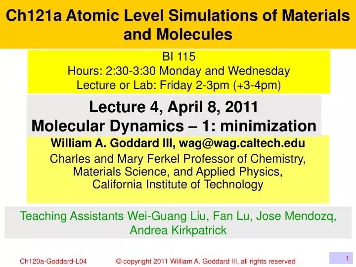
Ch121a Atomic Level Simulations of Materials and Molecules. BI 115 Hours: 2:30-3:30 Monday and Wednesday Lecture or Lab: Friday 2-3pm (+3-4pm). Lecture 4, April 8, 2011 Molecular Dynamics – 1: minimization. William A. Goddard III, wag@wag.caltech.edu

E N D
Ch121a Atomic Level Simulations of Materials and Molecules BI 115 Hours: 2:30-3:30 Monday and Wednesday Lecture or Lab: Friday 2-3pm (+3-4pm) Lecture 4, April 8, 2011 Molecular Dynamics – 1: minimization William A. Goddard III, wag@wag.caltech.edu Charles and Mary Ferkel Professor of Chemistry, Materials Science, and Applied Physics, California Institute of Technology Teaching Assistants Wei-Guang Liu, Fan Lu, Jose Mendozq, Andrea Kirkpatrick
Now that we have a FF, what do we do with it? Calculate the optimum geometry Calculate the vibrational spectra Do molecular dynamics simulations Calculate free energies, entropies, phase diagrams …..
Energy minimization Newton’s Method – 1D Expanding the energy expression about x0, we can write E(d) = E0 + d E0’ + ½ d2 E0” + O(d3) Where E’= (dE/dx)x0 and E” = (d2E/dx2)x0 at x0. At an energy minimum we have E’(dmin) = E0’ + dmin E0” = 0 and hence dmin =– E0’/E0” Thus give E0’ and E0” at point x0 we can estimate the minimum. If E(x) is parabolic this will be the exact Minimum. This is called Newton’s method Of course, E(x) may not be exactly parabolic. But then we recalculate E1’ and E1” at point 1 and estimate the minimum to be at x2 = x1 – E1’/E1”, This process converges quadratically. That is the error at each iteration is the square of the previous error. E x0 xmin x
More on Newton’s Method – 1D Newton’s method will rapidly locate the nearest local minimum if E” > 0. Note in the illustration, that this may not be the global minimum, which is at x2min. Also, if E” < 0 (eg. Between the green lines) Newton’s method takes us to a maximum rather than a minimum E x0 xmin x2min x
Energy minimization – 1D – no E” Now consider that we only know the slope, not the 2nd derivative. We start at point x0 of a one dimensional system, E(x), and want to find the minimum, xmin=x0 + dx Given the slope, E’=(dE/dx)x0 we know which way to go, but not how far. E x0 x1 Clearly we want dx = - lE’ That is we move in the direction opposite the slope, E’, but how far? With just E’, we cannot know. Thus we could pick some initial value l1 xmin x and evaluate the energy E1 and slope E1’ at the new point. If the new E1’ has the opposite slope, then we have bounded the minimum, and we can fit a parabola to estimate the minimum xmin = x0 – E0’/k where k= (E1’ – E0’)/(x1-x0) is the curvature of this parabola.
Energy minimization – one dimensional We would then evaluate E(xmin) to make sure that both points were in the same valley (and not x2). In the case that the 2nd point was x3, no change in slope, then we want to jump farther until E’ changes sign so that the minimum is bounded. E x0 xmin x3 In the case that the 2nd point was x2, then the new energy would not match the prediction based on the parabola. x2 x In this case we would choose whichever point of x0, xmin, and x2 had the lowest energy and we would use the E’ to choose the direction, but we would choose the jump, l, to be much smaller, say a factor of 2 than before (some people like using the Golden Mean of 2/[sqrt(5)-1] = 1.6180)
Energy minimization - multidimensional Consider a molecule with N atoms (J=1,N), It has 3N degrees of freedom (Ja, 1x to Nz) where a =x,y,z Denote these 3N coordinates as a vector, R. The energy is then E(R) Starting with an initial geometry, R0, consider the new geometry, Rnew = R0 + dR, and expand in a Taylor series E(Rnew)=E(R0)+Sk(dR)k(∂E/∂Rk)+½Sk,m(dR)k(dR)m(∂2E/∂Rk∂Rm) +O(d3) Writing the the energy gradient as E = (∂E/∂Rk) and the Hessian tensor as H=2E = (∂2E/∂Rk∂Rm) This becomes E(Rnew)=E(R0)+ (dR)∙E + ½(dR)∙H∙(dR) + O(d3)
Newton Raphson method in 3N space Given E(Rnew)=E(R0)+ (dR)∙E + ½(dR)∙H∙(dR) The condition that Rnew = R0 + dR lead to a minimum is that E + H∙(dR) = 0 Bearing in mind that His a matrix, the solution is (dR) = - (H)-1∙E where (H)-1is the inverse ofH This is exactly analogous to Newton’s method in 1D dmin =– E0’/E0” and in multidimensions it is called Newton-Raphson (NR) method. There are a number of practical issues with NR. First for Hb, with 6000 atoms the Hessian matrix would be of dimensions 18000 by 18000 and hence quite tedious to solve or even to store. First we must be sure that all eigenvalues of the Hessian are nonzero, since otherwise the inverse will be infinite. Such zero eigenvalues might seem implausible. But for a finite molecule with 3 or more atoms there are always 6 zero modes.
Hessian problems For example, translating all atoms of finite molecule by a finite distance in the x, y, or z directions cannot change the energy. In addition rotating a nonlinear molecule about either the x, y, or z axis cannot change the energy. Thus we must remove these 6 dof from the Hessian, reducing it to a (3N-6) by (3N-6) matrix before inverting it For a linear molecule, there are only 2 rotational modes, but if there are more than 2 atoms (say CO2) the dynamics will almost always lead to nonlinear structures, so we must consider 3N-6 dof. However for diatomics, there is only one nonzero eigenvalue (Bond stretch) Also all (3N-6) eigenvalues of the Hessian must be positive, otherwise NR will lead to a stationary point that is a maximum for some directions.
Steepest descents – 1st point Generally it is impractical to evaluate and diagonalize the Hessian matrix, thus we must make do with just, E, the gradient in 3N dimensions (no need to separate out translation or rotation since there will be no forces for these combinations of coordinates). Obviously, it would be best to move along the direction with the largest negative slope, this is called the steepest descent direction, u = -E/|E|, where u is a unit vector parallel with the vector E but pointed downhill. Then dR = l u, where l is a scalar Just as in 1D, we do not know how far to move, so we pick some value, l, and evaluate E1 at the new point. Of course E1 will generally have a component along u,(u∙E1) plus a component perpendicular to u. Here we proceed just as in the 1D case to bound the minimum and predict the minimum energy along the path
Steepest descents – more on 1st point Regarding the first l, Newton’s method suggests that it be L = 1/k where k is an average force constant (curvature in the E direction). In biograf/polygraf/ceriusII I used a value of k=200 as a generally good guess. Also note from the discussion of the 1D case, we want the first point to overshoot the minimum a bit so that the slope is positive. This way we can calculate k from the two slopes and predict a refined minimum. At the predicted minimum, we evaluate the slope in the original steepest descent direction and if it is small enough (significantly smaller than the other 2 slopes) and if the new energy is lower than the original energy, we use the new point to predict a new search direction
Steepest descents – 2nd point Starting from our original point x0 with slope E0, we moved in the direction, u0 = -E0/|E0| to find a final new position R1, along unit vector u0. Now we calculate E1 and a unit vector u1 = -E1/|E1|. If R1 was an exact minimum along unit vector u0then u1 will be orthogonal to u0. In the Steepest Descents (SD) method, we continue as for the 1st point to find the minimum R2 along unit vector u1, andthenthe minimum R3 along unit vector u2. The sequence of steps for SD is illustrated at the right. Here we see that the process of minimizing along u1, can result in no longer having a minimum along u0 u0 u0 u1 u1
Conjugate Gradients Even for a system like Hb with 18000 dof, the beharior shown in the SD figure is typcial, the system first minimizes along u0 then along u1, then back along u0 then back along u1, ignoring most of the other 18000 dof until the minimum in this 2D space is reached, at which point SD starts sampling other dof. The Conjugate Gradient method (Fletcher-Reeves) dramatically improves this process with little extra work. Here we define v1 = u1 – g u0 where g = (E1∙E1)/ (E0∙E0) (note the use of the dot or scalar product of the gradient vectors) Thus the new path v1combines both directions so that as we optimize along u1 we simultaneously keep the optimum along u0. (The ratio g is derived assuming that the energy surface is 2nd order.) This process is continued, with v2 = u2 – g u1 where g = (E2∙E2)/ (E1∙E1) The new E2 is perpendicular to all previous Ek.
Conjugate Gradients In 2D, for a system in which the energy changes quadratically, CG leads to the exact minimum in 2 steps, whereas SD would take many steps. First large systems, CG is the method of choice, unless the starting structure is really bad, in which case one might to SD for a few steps before starting CG. There reason is that CG is based on assuming that the energy x1 surface is quadratic so that the point is already in a valley and we want to find the optimum in that valley. SD is most appropriate when we start high up in the Alps and want to jump around to find a good valley, after which we can convert over to CG.
Fine points on CG • To ensure convergence, one must never choose a final point along a path higher than the original point defining the path. • If the final point is higher than the original point then it necessary to take the two lowest energy points and predict a third along the same path that is lower. • One must be careful if the first step does not find a change in sign of the slope along that path. One should predict the new minimum but if the predicted step is much larger (more thnan 10 times) than the original step, one should jump more cautiously. • With CG the fewest number of points along a pathway would be 1, so that the predict point is close enough to the minimum that a second checking point is not needed. • R. Fletcher and C.M. Reeves, Function minimization by congugate gradients, Computer Journal 7 (1964), 149-154 • Polak, B. and Ribiere, G. Note surla convergence des methode des directions conjuguees. Rev. Fr. Imform. Rech. Oper., 16, 35–43. (1969)
Inverse Hessian or Quasi-Newton methods In Newton-Raphson we choose the new point from (dR) = - (H)-1∙E where (H)-1is the inverse of the HessianH. For a system for which the energy is harmonic, this takes us directly to the minimum in one step Generally, it is too expensive to actually calculate and save the Hessian. However each time we search a path, say in CG, to find the minimum we derive an average force constant in that direction, k= (E1’ – E0’)/(x1-x0) where the gradients are projected along the path. Thus we can construct an approximate inverse Hessian which we assume initially to be the unit matrix (SG) but each time we minimize along a direction we use 1/k along this direction to improve our approximation to (H)-1.
Updating the Inverse Hessian The inverse Hessian, H is built up interatevely, AVOIDing explicitly inverting the Hessian matrix Hk= Inverse Hessian (H) approximation • Popular versions: • Davidson-Fletcher-Powell (DFS), • Broyden-Fletcher-Goldfarb-Shanno (BGFS), and • Murtaugh-Sargent (MS), are common [see Leach] - • These methods use only current and new points to update the inverse H • Better convergence achieved using more points (QM programs) 17-AJB
1st and 2nd Order Methods : Which to use? general rule of thumb: For large molecular systems with available analytical Force Field functions (1st and 2nd derivatives) Start with Steepest descent and switch to conjugate gradient after system is behaving rationally For small QM systems that are computationally expensive but for which second derivatives areunavailable Quasi-Newton methods
So Far … Gradient Based Methods Hold one solution at a time Look locally to see what direction to move in (gradient of the function at the current solution) Solution structure to closest minimum Select the new current solution after deciding how far to move along that path These methods are great for finding the local minimum but are not very useful The objective function is not smooth (i.e., not differentiable). There are multiple local minima. There are a large number of parameters. When the global minimum is desired
Global Minima Searchingwithout an exhaustive search !!! Note: No guaranteed analytical solution exists for most real (multivariate) applications in Molecular Simulations (MS) ! … but, closest (time-constrained) alternatives are: Random search algorithms Monte Carlo Simulated Annealing (adaptation of Metropolis-Hastings) Genetic Algorithms Molecular Dynamics • N. Metropolis, A.W. Rosenbluth, M.N. Rosenbluth, A.H. Teller, and E. Teller. "Equations of State Calculations by Fast Computing Machines". Journal of Chemical Physics, 21(6):1087-1092, 1953. • W.K. Hastings. "Monte Carlo Sampling Methods Using Markov Chains and Their Applications", Biometrika, 57(1):97-109, 1970 20-AJB
Stochastic Search Algorithms • The Totally Random Algorithm: • generates random parameter vectors • evaluates each one, and • saves the best one that it finds • Monte Carlo and Simulated Annealing (SA) approaches: • From one solution or time take a random step away from it. • If step results in a better solution, then it becomes the new solution about which random steps are taken. • As optimization proceeds, average size of steps decreases (system “cools” down). • Genetic Algorithms (GAs) • GAs contain a “population” of solutions at any one time. • 3 Step process: • A way to select parents (pop. generation and selection) • A mating ritual between the parents (genetics) • A survival of the fittest mechanism (a fitness measure) 21-AJB
Simulated Annealing A generalization of MC method for examining EOS and frozen states of n-body systems [metropolis et al, 1953] By Thermodynamics Analogy (liquids or metals): a melt, initially at high T and disordered, is slowly cooled (i.e. approximately at thermodynamics equilibrium at any time). As cooling proceeds, system becomes more ordered and approaches a “frozen” ground state at T=0. This reduces defects (induces softness, relieves internal stresses, refines the structure and improves cold working properties of metal). If initial T is too low or cooling is done insufficiently slowly the system may become quenched forming defects or freezing out in metastable states (ie. trapped in a local minimum energy state). Concept: at higher T more configuration become available !! Ground state E S. Kirkpatrick; C. D. Gelatt; M. P. Vecchi, Optimization by Simulated Annealing Science, New Series, Vol. 220, No. 4598. (May 13, 1983), pp. 671-680. 22-AJB
EM: Simulated AnnealingAlgorithm for EM in MS Start with system at a known configuration (E) T=hot Frozen=False While (!Frozen): Do Until Thermal Equilibrium @T Perturb system slightly (e.g. move particles) Compute ΔE=Enew-Ecurrent due to perturbation If (ΔE < 0) THEN Accept perturbation (new system configuration) Else Accept “maybe” with probability=exp(- ΔE/ KBT) If ΔE decreasing over last few T’s THEN: T=(1-ε)T (Cooling schedule) Else Frozen=True Return final configuration as low E solution HOT T1 Uphill moves “acceptable” at high T T2 Involves MD steps A T3 COLD Unreachable from A at T2 and T3 T1>T2>T3 • Cooling schedule critical: • Speed of convergence • Quality of minimum • Linear, exponent, sigmoid, etc. As SA progresses the system approaches ground state (T=0)
Genetic Algorithms (GAs) • Start global minima search with GA: • Establish numerical range for conformation variables (e.g. Angles, torsions, etc.) • Divide range by 2(n-1) intervals (n -> desired resolution) • Associate each slot with a configuration value (real) or use it to binary code the value (bin) • Generate binary representations of the individual variables stochastically, and combine them in a single binary string (position in string indicates parameter associated) • Generate a whole population • Calculate E for each state and determine conformation fit number • Optimize (adapt) • Generate new fitter offspring set (populations) by exchanging bits from parents - crossover • To avoid suboptimal solution (local minima) induce “mutations” by inverting randomly selected bits (every so often) • When GA pop. stops improving, switch to CG Fitness: Lowest E crossover mutation 24-AJB Implementations: Gromos, CMDF
EM: Convergence criteria Exact location of minima and saddle points are rare in real molecular modeling applications - so minimization would continue indefinitely. Need to terminate the process ! Energy difference between successive iterations RMS coordinates (change in successive conformations) RMS of gradient (recommended) GPCR-Helix CMDF CG-SP RMS 0.01 N_iter N_func Energy(kcal/mol) Energy_diff RMS_coords RMS_force 0 1 6.5678589836e+02 0.0000000000e+00 0.0000000000e+00 2.0609801246e+01 10 21 3.2995541076e+02 -6.8361848793e-04 6.3709030512e-05 1.6146775176e+00 20 42 3.2181491846e+02 -4.0985875833e-02 7.9228816836e-04 6.8419176497e-01 30 62 3.1691279419e+02 -1.3937305058e-02 5.2899529600e-04 7.0901724185e-01 40 82 3.1430948951e+02 -1.4732246578e-02 6.4474518504e-04 6.0462436581e-01 50 102 3.1251982226e+02 -7.6510768008e-04 1.6604142969e-04 4.9186883205e-01 60 122 3.1094106944e+02 -1.9026408838e-03 3.2189517910e-04 4.8629507807e-01 70 142 3.0969619774e+02 3.1197365510e-02 1.1929026568e-03 3.2359649746e-01 80 162 3.0863355352e+02 -1.3188847153e-03 2.7051239481e-04 3.5778184685e-01 90 182 3.0774713732e+02 9.9227506212e-06 8.0820179633e-05 3.3577681153e-01 99 201 3.0715578558e+02 -2.4492005913e-03 2.6292140614e-04 3.9285171778e-01 Total energy= 3.0715578558e+02 nflag = 1, total N_iterations = 99, total N_function_calls = 201
Vibration Consider Newton’s equation for a spring M (d2x/dt2) = F = -k (x-xe) Assume x-x0=d = A cos(wt) then –Mw2 Acos(wt) = -k A cos(wt) Hence w = Sqrt(k/M). Stiffer force constant higher w and higher M lower w Now generalize to M dof Fk = -(∂E(Rnew)/∂Rk) = -(∂E/∂Rk) - Sm (∂2E/∂Rk∂Rm) (dR)m Assuming that we take the equilibrium position as our reference, then the first term 0, so we get Fk = - Sm Hkm (dR)m = Mk (∂2Rk)/∂t2) Again assuming (dR)m = Am cos wt we get Mk(∂2Rk)/∂t2) = Mkw2 (Ak cos wt) = Sm Hkm (Amcos wt) Thus the coefficient of cos wt must be zero {Mkw2 Ak - Sm Hkm Am}=0
Solving for the Vibrational modes The normal modes satisfy {Mkw2 Ak - Sm Hkm Am}=0 Writing Bk = sqrt(Mk)Ak we get Sm Gkm Bm = w2 Bk where Gkm = Hkm/sqrt(MkMm) where G is referred to as the reduced Hessian For M degrees of freedom this has M eigenstates Sm Gkm Bmp = dkp Bk (w2)p where the eigenvalues are the squares of the vibrational energies. Note that if the point of interest were not a minimum, but say a saddle point with one negative curvature, G would have one negative eigenvalue leading to an imaginary frequency If the Hessian includes the 6 translation and rotation modes then there will be 6 zero frequency modes
Thermodynamics using vibrational partition function with vibrational modes
Using the vibrational modes: thermodynamics In QM and MM Energy at minima = motionless state at 0K BUT, experiments are made at finite T, hence corrections are required to allow for rotational, translational and vibrational motion. The internal energy of the system: U(T)=Urot(T)+Utran(T)+Uvib(T)+Uvib(0) • From equipartition theorem: Urot(T) and Utran(T) are both equal to (3/2)KBT per molecule (except Urot(T)=KBT for linear molecules) • BUT, vibrational energy levels are often only partially excited at room T, thus Uvib(T) requires knowledge of vibrational frequencies • Uvib(T) = vibrational enthalpy @ T - vibrational enthalpy @ 0K Vibrational frequencies can be used to calculate entropies and free energies, or to compare with results of spectroscopic experiments The vibrational frequencies (νi) of the normal modes (Nmod) calculated from the eigenvalues (λi) of the force-constant equivalent of Hessian matrix of second derivatives 29-AJB
MM: Saddle Points and Minima from Hessian Example function f(x,y)=x4+4x2y2-2x2+2y2 f’(x,y)=[(4x2+8y2-4)x,(8x2+4)y] f’ = 0 at (1,0);(0,0);(-1,0) Both eigenvalues are positive: (1,0) and (-1,0) are a minima One positive and one negative eigenvalue: (0,0) is a saddle point 30-AJB
MM: Transition Structures and Reaction Pathways From a chemical process we require: Thermodynamics (relative stability of species) -> minimum points on PES Kinetics (rate of conversion from one structure to another) -> nature of PES away from minimum points (e.g. path between 2 minima = “reaction” pathway). Example: Gas-phase reaction between chloride ion (Cl-) and methyl chloride (CH3Cl). As the chloride ion approaches the methyl chloride along the C-Cl bond the E passes through an ion-dipole complex which is at a minimum. The energy then rises to a max at the pentagonal transition state. Transition structure 31-AJB Adapted from Chandrasekhar J, S.F. Smith and W.L. Jorgensen, JACS, 107, 1985
Summary Energy Minimization and Conformational Analysis (use FF) Transition structures and Reaction pathways distinguishing minima, maxima and saddle points Normal modes analysis (use Hessian) Deriving partition function to determine thermodynamics properties (only for small systems) … need something else -> MD (next) Demos with Lingraf, CMDF and LAMMPS
MM: Recap and Highlights Each particle assigned: radius (vdW), polarizability, and constant net charge (generally derived from quantum calculations and/or experiment) Interactions pre-assigned to specific sets of atoms. Bonded interactions are conventionally treated as "springs" (equilibrium -> experimental or QM) Interactions determine the spatial distribution of atom-like particles and their energies. PES leads to Force Fields (FF) Which FF to use depends on: Type of bond modeled (E.g. metallic, covalent, ionic, etc) Desired precision (E.g. Chemistry vs. Statistical Mechanics) Desired transferability (E.g. Describe multiple bond types) Size and time of system simulation Available computational resources structures of isolated molecules can lead to misleading conclusions (full interactions MUST be considered, e.g. solvent)
Related Reading Material and Molecular Simulation Codes Books and Manuals Andrew W. Leach, Molecular Modeling: Principles and Applications, 2nd Ed., Prentice Hall 2001. Chapters: 4, and 5 Dean Frenkel and Berend Smit, Understanding Molecular Simulation: From Algorithms to Applications, Academic Press, 2002. Chapters: 4 and 6 Polygraph (Reference Manual, Appendix G, Force Fields) Software: LAMMPS (http://lammps.sandia.gov/) Lingraf (https://wiki.wag.caltech.edu/twiki/bin/view/Main/LingrafPage) CMDF (https://wiki.wag.caltech.edu/twiki/bin/view/CMDF/WebHome) Cerius2 (http://www.accelrys.com/products/cerius2/).
Problem Set 1-16/26-2009 Energy minimization is used to determine stable states for a molecular structure. Using Lingraf, minimize a tripeptide (e.g. Glutathione or a Thyrotropin-releasing hormone) to an RMS force of 0.01 molecule with: Steepest Descent (v145) Conjugate Gradient (v200) Fletcher-Powel Conjugate Gradient (v200) Annealed Dynamics with: 1 annealing cycle using standard microcanonical dynamics per cycle, and a temperature profile starting at 100K and ending at 0K. Minimize after annealed dynamics. Write down results for: Number of minimization steps Converged (if) Energy Value Explain your results IR spectroscopy is used as a qualitative analysis tool for sample identification. IR data is used to help determine molecular structure.The absorption/transmission of infrared (IR) light by a molecule causes excitation of the vibrational motions of the atoms present. Different types of bonds in the molecule will absorb light of different wavelengths, thus allowing qualitative identification of certain bond types in the sample. A first step towards calculating the IR spectrum (say in, transmission mode) of a molecule using MM techniques involves computing its vibrational frequencies; this can be done from the Hessian of second derivatives of the corresponding potential energy surface for the system. What would be required to determine the full IR spectrum (transmission mode) once we’ve obtained the vibrations?. Please explain and elaborate on a proposed mathematical framework for doing so. Choose a very simple molecule for which the IR spectra has been experimentally characterized (e.g ethylene monomer, in any medium). Use Lingraf to construct the molecule and to calculate its vibrational modes, frequencies and the IR spectra. Interpet your findings in terms of molecular composition. Compare your results with the experimental values referenced; explain any differences.