Download
1 / 25
260 likes | 402 Views
Section 12-1. Visual Displays of Data. Visual Displays of Data. Basic Concepts Frequency Distributions Grouped Frequency Distributions Stem-and-Leaf Displays Bar Graphs, Circle Graphs, and Line Graphs. Basic Concepts.

E N D
Section 12-1 • Visual Displays of Data
Visual Displays of Data • Basic Concepts • Frequency Distributions • Grouped Frequency Distributions • Stem-and-Leaf Displays • Bar Graphs, Circle Graphs, and Line Graphs
Basic Concepts In statistics a population, includes all of the items of interest, and a sample, includes some of the items in the population. The study of statistics can be divided into two main areas. Descriptive statistics, has to do with collecting, organizing, summarizing, and presenting data (information). Inferential statistics, has to do with drawing inferences or conclusions about populations based on information from samples.
Basic Concepts Information that has been collected but not yet organized or processed is called raw data. It is often quantitative (or numerical), but can also be qualitative (or nonnumerical).
Basic Concepts Quantitative data: The number of siblings in ten different families: 3, 1, 2, 1, 5, 4, 3, 3, 8, 2 Qualitative data: The makes of five different automobiles: Toyota, Ford, Nissan, Chevrolet, Honda Quantitative data can be sorted in mathematical order. The number siblings can appear as 1, 1, 2, 2, 3, 3, 3, 4, 5, 8
Frequency Distributions When a data set includes many repeated items, it can be organized into a frequency distribution, which lists the distinct values (x) along with their frequencies (f ). It is also helpful to show the relative frequency of each distinct item. This is the fraction, or percentage, of the data set represented by each item.
Example: Frequency Distribution The ten students in a math class were polled as to the number of siblings in their individual families. Construct a frequency distribution and a relative frequency distribution for the responses below. 3, 2, 2, 1, 3, 4, 3, 3, 4, 2
Example: Frequency Distribution Solution
Histogram The data from the previous example can be interpreted with the aid of a histogram. A series of rectangles, whose lengths represent the frequencies, are placed next to each other as shown below. Frequency Siblings
Frequency Polygon The information can also be conveyed by a frequency polygon. Simply plot a single point at the appropriate height for each frequency, connect the points with a series of connected line segments and complete the polygon with segments that trail down to the axis. Frequency Siblings
Line Graph The frequency polygon is an instance of the more general line graph. Frequency Siblings
Grouped Frequency Distributions Data sets containing large numbers of items are often arranged into groups, or classes. All data items are assigned to their appropriate classes, and then a grouped frequency distribution can be set up and a graph displayed.
Guidelines for the Classes of a Grouped Frequency Distribution 1. Make sure each data item will fit into one and only one, class. 2. Try to make all the classes the same width. 3. Make sure that the classes do not overlap. 4. Use from 5 to 12 classes.
Example: Frequency Distribution Twenty students, selected randomly were asked to estimate the number of hours that they had spent studying in the past week (in and out of class). The responses are recorded below. 15 58 37 42 20 27 36 57 29 42 51 28 46 29 58 55 43 40 56 36 Tabulate a grouped frequency distribution and a relative frequency distribution and construct a histogram for the given data.
Example: Frequency Distribution Solution
Example: Histogram of Data Solution(continued) Frequency 10-19 20-29 30-39 40-49 50-59 Hours
Frequency Distribution In the table, the numbers 10, 20, 30, 40, and 50 are called the lower class limits. They are the smallest possible data values within their respective classes. The numbers 19, 29, 39, 49, and 59 are called the upper class limits. The class width for the distribution is the difference of any two successive lower (or upper) class limits. In this case the class width is 10.
Stem-and-Leaf Displays The tens digits to the left of the vertical line, are the “stems,” while the corresponding ones digits are the “leaves.” The stem and leaf conveys the impressions that a histogram would without a drawing. It also preserves the exact data values.
Example: Stem-and-Leaf Displays Below is a stem-and-leaf display of the data from the last example (15 58 37 42 20 27 36 57 29 42 51 28 46 29 58 55 43 40 56 36)
Bar Graphs A frequency distribution of nonnumerical observations can be presented in the form of a bar graph, which is similar to a histogram except that the rectangles (bars) usually are not touching each one another and sometimes are arranged horizontally rather than vertically.
Example: Bar Graph A bar graph is given for the occurrence of vowels in this sentence. Frequency A E I O U Vowel
Circle Graphs A graphical alternative to the bar graph is the circle graph, or pie chart, which uses a circle to represent all the categories and divides the circle into sectors, or wedges (like pieces of pie), whose sizes show the relative magnitude of the categories. The angle around the entire circle measures 360°. For example, a category representing 20% of the whole should correspond to a sector whose central angle is 20% of 360° which is 72°.
Example: Expenses A general estimate of Amy’s monthly expenses are illustrated in the circle graph below. Clothing 10% Other 35% Rent25% Food 30%
Line Graph If we are interested in demonstrating how a quantity changes, say with respect to time, we use a line graph. We connect a series of segments that rise and fall with time, according to the magnitude of the quantity being illustrated.
Example: Line Graph The line graph below shows the stock price of company PCWP over a 6-month span. Price in dollars Jan Feb Mar Apr May June Month