Download
1 / 38
380 likes | 602 Views
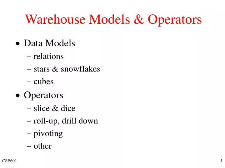
Warehouse Models & Operators. Data Models relations stars & snowflakes cubes Operators slice & dice roll-up, drill down pivoting other. Multi-Dimensional Data. Measures - numerical (and additive) data being tracked in business, can be analyzed a nd examined

E N D
Warehouse Models & Operators • Data Models • relations • stars & snowflakes • cubes • Operators • slice & dice • roll-up, drill down • pivoting • other CSE601
Multi-Dimensional Data • Measures - numerical (and additive) data being tracked in business, can be analyzed and examined • Dimensions - business parameters that define a transaction, relatively static data such as lookup or reference tables • Example: Analyst may want to view sales data (measure) by geography, by time, and by product (dimensions) CSE601
“Sales by product line over the past six months” “Sales by store between 1990 and 1995” The Multi-Dimensional Model Store Info Key columns joining fact table to dimension tables Numerical Measures Prod Code Time Code Store Code Sales Qty Fact table for measures Product Info Dimension tables Time Info . . . CSE601
Multidimensional Modeling • Multidimensional modeling is a technique for structuring data around the business concepts • ER models describe “entities” and “relationships” • Multidimensional models describe “measures” and “dimensions” CSE601
Dimensions are organized into hierarchies E.g., Time dimension: days weeks quarters E.g., Product dimension: product product line brand Dimensions have attributes Time Store Dimensional Modeling Date Month Year StoreID City State Country Region CSE601
Dimension Hierarchies Store Dimension Product Dimension Total Total Region Manufacturer District Brand Stores Products CSE601
Schema Design • Most data warehouses use a star schema to represent multi-dimensional model. • Each dimension is represented by a dimension table that describes it. • A fact table connects to all dimension tables with a multiple join. Each tuple in the fact table consists of a pointer to each of the dimension tables that provide its multi-dimensional coordinates and stores measures for those coordinates. • The links between the fact table in the center and the dimension tables in the extremities form a shape like a star. CSE601
Star Schema (in RDBMS) CSE601
Star Schema Example CSE601
Star Schema with Sample Data CSE601
The “Classic” Star Schema • A relational model with a one-to-many relationship between dimension table and fact table. • A single fact table, with detail and summary data • Fact table primary key has only one key column per dimension • Each dimension is a single table, highly denormalized • Benefits: Easy to understand, intuitive mapping between the business entities, easy to define hierarchies, reduces # of physical joins, low maintenance, very simple metadata • Drawbacks: Summary data in the fact table yields poorer performance for summary levels, huge dimension tables a problem CSE601
Need for Aggregates • Sizes of typical tables: • Time dimension: 5 years x 365 days = 1825 • Store dimension: 300 stores reporting daily sales • Production dimension: 40,000 products in each store (about 4000 sell in each store daily) • Maximum number of base fact table records: 2 billion (lowest level of detail) • A query involving 1 brand, all store, 1 year: retrieve/summarize over 7 million fact table rows. CSE601
Aggregating Fact Tables • Aggregate fact tables are summaries of the most granular data at higher levels along the dimension hierarchies. Hierarchy levels Product key Product Category Department Store key Store name Territory Region Product key Time key Store key Unit sales Sale dollars Multi-way aggregates: Territory – Category – Month Time key Date Month Quarter Year (Data values at higher level) CSE601
The “Fact Constellation” Schema District Fact Table Region Fact Table District_ID PRODUCT_KEY PERIOD_KEY Region_ID PRODUCT_KEY PERIOD_KEY Dollars Units Price Dollars Units Price CSE601
Aggregate Fact Tables Store Product Base table Sales facts Store key Store name Territory Region Product key Product Category Department Product key Time key Store key Unit sales Sale dollars Dimension Derived from Product Category Time One-way aggregate Sale facts Time key Date Month Quarter Year Category key Category Department Category key Time key Store key Unit sales Sales dollars CSE601
Families of Stars Dimension table Dimension table Dimension table Fact table Fact table Dimension table Dimension table Fact table Dimension table Dimension table Dimension table CSE601
Snowflake Schema • Snowflake schema is a type of star schema but a more complex model. • “Snowflaking” is a method of normalizing the dimension tables in a star schema. • The normalization eliminates redundancy. • The result is more complex queries and reduced query performance. CSE601
Sales: Snowflake Schema Category key Product category Brand key Brand name Category key Region key Region name Product key Product name Product code Brand key Territory key Territory name Region key Sales fact Product key Time key Customer key …. Salesrep key Salesperson name Territory key Product Salesrep CSE601
Snowflaking • The attributes with low cardinality in each original dimension table are removed to form separate tables. These new tables are linked back to the original dimension table through artificial keys. Product key Product name Product code Brand key Brand key Brand name Category key Category key Product category CSE601
Snowflake Schema • Advantages: • Small saving in storage space • Normalized structures are easier to update and maintain • Disadvantages: • Schema less intuitive and end-users are put off by the complexity • Ability to browse through the contents difficult • Degrade query performance because of additional joins CSE601
What is the Best Design? • Performance benchmarking can be used to determine what is the best design. • Snowflake schema: easier to maintain dimension tables when dimension tables are very large (reduce overall space). It is not generally recommended in a data warehouse environment. • Star schema: more effective for data cube browsing (less joins): can affect performance. CSE601
Aggregates • Add up amounts for day 1 • In SQL: SELECT sum(amt) FROM SALE WHERE date = 1 81 CSE601
Aggregates • Add up amounts by day • In SQL: SELECT date, sum(amt) FROM SALE GROUP BY date CSE601
Another Example • Add up amounts by day, product • In SQL: SELECT date, sum(amt) FROM SALE • GROUP BY date, prodId rollup drill-down CSE601
Aggregates • Operators: sum, count, max, min, median, ave • “Having” clause • Using dimension hierarchy • average by region (within store) • maximum by month (within date) CSE601
Data Cube Fact table view: Multi-dimensional cube: dimensions = 2 CSE601
3-D Cube Fact table view: Multi-dimensional cube: day 2 day 1 dimensions = 3 CSE601
Example roll-up to region Dimensions: Time, Product, Store Attributes: Product (upc, price, …) Store … … Hierarchies: Product Brand … Day Week Quarter Store Region Country NY Store SF roll-up to brand LA 10 34 56 32 12 56 Juice Milk Coke Cream Soap Bread Product roll-up to week M T W Th F S S Time 56 units of bread sold in LA on M CSE601
Cube Aggregation: Roll-up rollup drill-down Example: computing sums day 2 . . . day 1 129 CSE601
Cube Operators for Roll-up day 2 . . . day 1 sale(s1,*,*) 129 sale(s2,p2,*) sale(*,*,*) CSE601
Extended Cube * day 2 sale(*,p2,*) day 1 CSE601
Aggregation Using Hierarchies store day 2 day 1 region country (store s1 in Region A; stores s2, s3 in Region B) CSE601
Slicing day 2 day 1 TIME = day 1 CSE601
Slicing & Pivoting CSE601
Summary of Operations • Aggregation (roll-up) • aggregate (summarize) data to the next higher dimension element • e.g., total sales by city, year total sales by region, year • Navigation to detailed data (drill-down) • Selection (slice) defines a subcube • e.g., sales where city =‘Gainesville’ and date = ‘1/15/90’ • Calculation and ranking • e.g., top 3% of cities by average income • Visualization operations (e.g., Pivot) • Time functions • e.g., time average CSE601
Query & Analysis Tools • Query Building • Report Writers (comparisons, growth, graphs,…) • Spreadsheet Systems • Web Interfaces • Data Mining CSE601
Implementation of OLAP Server • ROLAP: relational OLAP – data are stored in tables in relational databases or extended-relational databases. They use an RDBMS to manage the warehouse data and aggregations using often a star schema. • They support extensions to SQL. • A cell in the multi-dimensional structure is represented by a tuple. • Advantage: scalable (no empty cells for sparse cube). • Disadvantage: no direct access to cells. CSE601
Implementation of OLAP Server • MOLAP: multidimensional OLAP – implements the multidimensional view by storing data in special multidimensional data structure (MDDS). • Advantage: fast indexing to pre-computed aggregations. Only values are stored. • Disadvantage: not very scalable and sparse. CSE601