Download
1 / 34
410 likes | 585 Views
Dynamics of Robot Manipulators. Purpose:

E N D
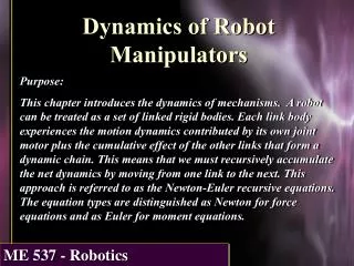
Dynamics of Robot Manipulators Purpose: This chapter introduces the dynamics of mechanisms. A robot can be treated as a set of linked rigid bodies. Each link body experiences the motion dynamics contributed by its own joint motor plus the cumulative effect of the other links that form a dynamic chain. This means that we must recursively accumulate the net dynamics by moving from one link to the next. This approach is referred to as the Newton-Euler recursive equations. The equation types are distinguished as Newton for force equations and as Euler for moment equations.
In particular, you will • Review the fundamental force and moment equations for rigid bodies. • Determine that the moment of forces applied to a rigid body is the rate of change of angular momentum if taken about the body’s center of mass or about an inertial point. • Apply Newton-Euler recursive equations for the connected rigid links of a mechanism. • Understand that forward recursion is used to propagate motion through the links, while backward recursion is used to propagate forces and torques through the links.
Given a system of particles translating through space, each particle i being acted upon by external force Fi, and each particle located relative to an inertial reference frame, the governing equations are Fc = m ac (6.10) M = (6.11) Mc = c (6.12) Review of fundamental equations What is an inertial frame?
Review of fundamental equations where m = total mass (sum over all mass particles) ac = acceleration of center of mass (cm) of all mass particles Fc = sum of external forces applied to system of particles as if applied at cm Hi = ri x mivi =angular momentum of particle i (also called moment of momentum) H, Hc = angular momentum summed over all particles, measured about inertial point, cm point, respectively M, Mc = moment of all external forces applied to system of particles, measured about inertial point, cm point, respectively
The time rate of change of any vector V capable of being viewed in either XYZ or xyz is [ ]XYZ = [ ]xyz + w x V where w is the angular velocity of a secondary translating, rotating reference frame (xyz). w z a y Z x Y X Rigid bodies in general motion (translating and rotating)
Another common form of the equation is: = r + w x V (6.13) and when applied to rate of change of angular momentum becomes M = = r + w x H (6.16) which is referred to as Euler’s equation. w z a y Z x Y X Rigid bodies in general motion (translating and rotating)
Rotating rigid body By integrating the motion over the rigid body, we can express the angular momentum relative to the xyz axes as H = Hx i + Hy j + Hz k = (Jxxwx + Jxywy + Jxzwz) i + (Jyxwx + Jyywy + Jyzwz) j + (Jzxwx + Jzywy + Jzzwz) k(6.20) products moments or in matrix form H = Jw where J = inertia matrix
Taking the derivative of (6.20) and substituting into (6.16), also assuming the body axes to be aligned with the principal axes, we get Euler’s moment equations: Mx = Jxxx + (Jzz - Jyy) wywz (6.29a) My = Jyyy + (Jxx - Jzz) wxwz (6.29b) Mz = Jzzz + (Jyy - Jxx) wxwy (6.29c) Rotating rigid body What are principal axes?
Acceleration relative to a non-inertial reference frame a w P z Z r y r R x Y X
Acceleration relative to a non-inertial reference frame By taking two derivatives and applying (6.13) appropriately, the absolute acceleration of point P can be shown to be a= + a x r + w x (w x r) + + 2 w x (6.31) where = acceleration of xyz origin a x r = tangential acceleration w x (w x r) = centripetal acceleration = acceleration of P relative to xyz 2 w x = Coriolis acceleration
Acceleration relative to a non-inertial reference frame For the special case of xyz fixed to rigid body and P a point in the body, and (6.31) reduces to a = + axr + wx (wxr) (6.32) If P at cm, then ac = + a x rc + wx (w x rc) (6.33)
Recursive Newton-Euler Equations (forward recursion for motion) Use Craig/Red D-H form
Recursive Newton-Euler Equations If vi = i and wi is defined to be the angular velocity of the ith joint frame xi yi zi with respect to base coordinates, then where describes the velocity of xi+1, yi+1, zi+1 relative to an observer in frame xi, yi, zi.
Recursive Newton-Euler Equations Likewise, the acceleration becomes Defining wi+1 to be the absolute angular velocity of the i+1 frame and to be the angular velocity of the i+1 frame relative to the ith frame:
Recursive Newton-Euler Equations Taking one more derivative for angular acceleration:
Recursive Newton-Euler Equations Now applying the DH coordinate representation for manipulators:
Recursive Newton-Euler Equations Using the previous equations, we can generate the angular motion recursive equations:
Recursive Newton-Euler Equations The linear velocity and acceleration equations use the D-H forms: where i+1 is the translational velocity of xi+1, yi+1, zi+1 relative to xi , yi , zi
Recursive Newton-Euler Equations Substituting (6.59) – (6.62), we get the velocity and acceleration recursion equations: Note that wi+1 = wi for translational link i+1.
w i . w i F i c i * w i p i Recursive Newton-Euler Equations (backward recursion for forces and torques) Joint i+1 Link i N z i i+1 , z i r Z i o Y o X o
Recursive Newton-Euler Equations (backward recursion for forces and torques) n i+1 f i+1 Link i f i n Joint Forces/Torques i
Recursive Newton-Euler Equations Define the terms: mi = mass of link i ri = position of link i cm with respect to base coordinates Fi = total force exerted on link i Ni = total moment " " " " * Ji = inertia matrix of link i about its cm determined in the Xo Yo Zo axes fi = force exerted on link i by link i-1 ni = moment " " " “
Recursive Newton-Euler Equations For each link we must apply the N-E equations: The gravitational acceleration and damping torques will be added to the equations of motion later.
Recursive Newton-Euler Equations Now i is easily calculated by knowing the acceleration of the origin of the ith frame attached to link i at joint i. We locate link i cm with respect to xi yi zi by ci such that ri = ci + pi. The velocity of the cm of link i is obviously
Recursive Newton-Euler Equations To determine Fi and Ni define fi = force exerted on link i by link i-1 ni = moment " " " “ Then Fi = fi – fi+1 (6.71) and Ni = ni – ni+1 + (pi - ri ) x fi - (pi+1 - ri ) x fi+1 (6.72) = ni – ni+1 - ci x Fi – si+1 x fi+1
Recursive Newton-Euler Equations The previous equations can be placed in the backwards recursion form to work from the forces/moments exerted on the hand backwards to the joint torques necessary to react to these hand interactions and move the manipulator: fi = fi+1 + Fi (6.74) ni = ni+1 + cix Fi + si+1x fi+1 + Ni (6.75)
Recursive Newton-Euler Equations The motor torque ti required at joint i is the sum of the joint torque ni resolved along the revolute axis plus the damping torque, ti = ni˙ zi+bii (revolute) (6.76a) where bi is the damping coefficient. For a translational joint ti = lifi˙zi + bii (translational) (6.77a) whereli is the torque arm for motor i.
The effect of gravity on each link is accounted for by applying a base acceleration equal to gravity to the base frame of the robot: o = g zo with zo vertical. o is applied to the base link in equations (6.65) and (6.66) for i = 0 and this serves to transmit the acceleration of gravity to each link by recursion. And what about gravity?
There are two basic problems with the derivation so far. What are they? Problem 1 - Ji in (6.68) when resolved into base coordinates is a function of manipulator configuration. To avoid this unnecessary complexity, we apply the equations at the cm of each link where Ji is constant. Problem 2 – The recursive relations have not resolved the various vectors from one joint frame to the next. We must adjust the equations accordingly.
We resolve the free vectors by applying the rotational sub-matrix of the D-H transformations for each joint frame to the recursive vectors, using the Craig/Red D-H representation. Let us also use Tsai’s notation. joint frame i+1 relative to joint frame i: joint frame i relative to joint frame i+1: Do we use the full homogeneous transformation in the recursive equations?
Revised angular motion equations Do you notice anything about the form of the D-H rotational sub-matrix?
Dynamics summary The N-E equations are applied recursively to generate the forces and torques at each joint motor. We first apply forward recursion to get the motion state for each link. We then use this motion state to propagate the forces and torques in backward recursion to each joint. The rotational sub-matrix of the D-H transformations must be applied to resolve the vectors correctly into each link’s joint frame .