Download
1 / 28
850 likes | 2.02k Views
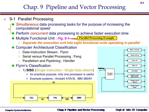
PIPELINE AND VECTOR PROCESSING. CHAPTER # 9. CONTENTS. Parallel Processing Pipelining Arithmetic Pipeline Instruction Pipeline RISC Pipeline Vector Processing Array Processors. Figure 9-1 Processor with multiple functional units. Adder-sub tractor. Integer multiply. Logic unit.

E N D
PIPELINE AND VECTOR PROCESSING CHAPTER # 9
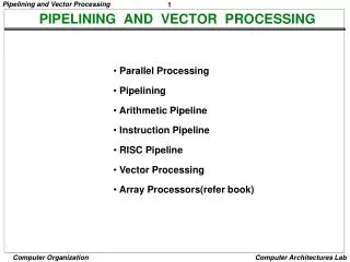
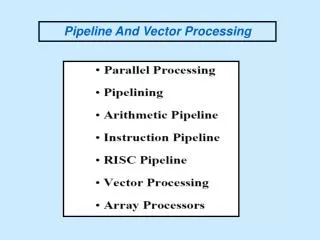
CONTENTS • Parallel Processing • Pipelining • Arithmetic Pipeline • Instruction Pipeline • RISC Pipeline • Vector Processing • Array Processors
Figure 9-1Processor with multiple functional units Adder-sub tractor Integer multiply Logic unit Shift unit Processor register Incrementer Floating-point Add-subtract Floating-point multiply Floating-point divide
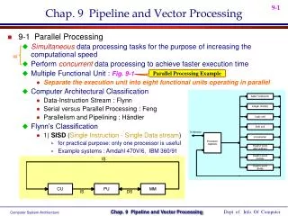
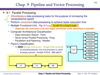
Instruction and stream. • Single instruction stream, single data stream (SISD). • Single instruction stream, multiple data stream (SIMD). • Multiple instruction stream, single data stream (MISD). • Multiple instruction stream, multiple data stream (MIMD).
Figure 9-2Example of Pipelining. Ai BiCi • R1 Ai , R2 Bi InputAiandBi • R3 R1* R2, R4Ci Multiply and input Ci • R5 R3 + R4 Add Ci to product R1 R2 Multiplier R4 R3 Adder R5
Table 9-1 Content of registers in pipeline example.
Figure 9-4Space-time diagram for pipeline. Clock cycle Segment: 1 2 3 4
Ii Ii+1 Ii+2 Ii+3 P1 P2 P3 P4 Figure 9-5Multiple functional units in parallel.
a b A B R R Difference Compare Exponent By subtraction Segment 1 Align mantissas R R R Segment 2 Choose exponent Add or subtract mantissas Segment 3 R R Normalize result Adjust Exponent Segment 4 R R Figure 9-6 Pipeline for floating-point and subtraction. Mantissas
Instruction Pipeline • Fetch the instruction from memory. • Decode the instruction. • Calculate the effective address. • Fetch the operands from memory. • Execute the instruction. • Store the result in the proper place.
Fetch instruction from memory Segment 1 Decode instruction And calculate Effective address Segment 2 yes Branch? no Fetch operand From memory Segment 3 Execute instruction Segment 4 yes Interrupt handling Interrupt? no Update PC Empty pipe Figure 9-7Four-segment CPU pipeline.
Figure 9-8Timing of instruction pipeline. Step: 1 2 3 4 5 6 7 8 9 11 12 13 10 Instruction: 1 FI DA FO EX 2 FI DA FO EX 3 FI DA FO EX (Branch) 4 EX FI -- -- FI DA FO 5 EX FI DA FO -- -- -- 6 EX FI DA FO 7 FO EX FI DA
Pipeline Conflicts • Resource conflicts • Data dependency conflicts • Branch difficulties conflicts
Delayed Load LOAD R1 M[address 1] LOAD R2 M[address 2] ADD R3 R1+R2 STORE M[address 3] R3
1 2 3 4 5 6 7 1 2 3 4 5 6 Clock cycles Clock cycles I E A I A E 1. Load R1 1. Load R1 I E A 2. Load R2 A E I 2. Load R2 I A E 3. No-operation I A E 3. Add R1+R2 A I E 4. Add R1+R2 4. StoreR3 5. StoreR3 I A E I A Pipeline timing with data conflict Pipeline timing with delayed load Figure 9-9Three segment pipeline timing. E
1 2 3 4 5 6 7 8 9 10 Clock cycles I A E 1. Load A E I 2. Increment I A E 3. Add 4. Subtract I A E 5. Branch to X I A E 6. NO-operation I A E 7. NO-operation I A E 8. Instruction in X A I E Figure 9-10Examples of delayed branch. Using no-operation instructions
Figure 9-10Examples of delayed branch. Clock cycles I A E 1. Load I A E 2. Increment I E 3. Branch to X A A I E 4. Add 5. Subtract A I E 6. Instruction in X E I A Rearranging instruction
Application of Vector Processing • Long range weather forecasting. • Petroleum explorations. • Seismic data analysis. • Medical diagnosis. • Aerodynamics and space flight simulations.
Figure 9-11Instruction format for vector processor Operation code Base address Source 1 Base address Source 2 Base address destination Vector length
Source A Multiplier pipeline Adder pipeline Source B Figure 9-12Pipeline for calculating an inner product
Address bus AR AR AR AR Memory array Memory array Memory array Memory array DR DR DR DR Data bus Figure 9-13Multiple module memory organization
Types of Array Processors • Attached Array Processor • SIMD Array Processor
General-Purpose computer input-output interface Attached array processor Main memory High-speed memory to Local memory Memory bus Figure 9-14Attached Array Processor with host computer
PE1 M1 Master control unit PE2 M2 PE3 M3 Main memory PEn Mn Figure 9-15SIMD array processor organization