Download
1 / 19
190 likes | 298 Views
Injection height for biomass burning emissions from boreal forest fires.

E N D
Injection height for biomass burning emissions from boreal forest fires On opponents of greenhouse gas abatement: "Your political base will melt away as surely as the polar ice caps... You will become a political penguin on a smaller and smaller ice floe that is drifting out to sea. Goodbye, my little friend! That's what's going to happen." – Arnold Schwarzenegger Fok-Yan Leung April 12, 2007. Harvard University Special thanks to: Jennifer Logan, Rokjin Park, and Dominic Spracklen (Harvard) Edward Hyer and Eric Kasischke (UMD) Leonid Yurganov David Diner, Dominic Mazzoni, David Nelson, and Ralph Kahn (NASA/JPL) Funding from the NSF and EPA
We began by looking at emissions estimates for 1998 boreal fires, which vary significantly. Discrepancies between KAS05 and KAJ02 stem primarily from differences in assumptions about belowground burning KAS05 emissions 2x as large as KAJ02 emissions KAJ02 emissions “Interannual” emissions Derived using TOMS-AI (for 1998) “Climatological” emissions
Comparison of surface and column data from 1998 with results of GEOS-Chem simulations KAJ02 emissions KAJ02 emissions baseline emissions KAS05 emissions data - average data - 1998
During intense boreal fires, intense heat can result in lofting of emissions well above the boundary layer • In GEOS-Chem, all biomass burning emissions are injected in boundary layer by default. • Base initial parameterization on assumptions that: • The majority of emissions from crown fires are more likely to be lofted into the free troposphere. • Crown fires are prevalent during highest burning months • Based on the above, and the work of Kasischke, (2005), we injected: • 40% of all emissions in boundary layer • 60% into free troposphere
Putting large fraction of emissions in free troposphere reconciled model results with both surface and column data • For both surface and column data (anomaly data): KAS05 seems to perform better in capturing the CO behavior using parameterization KAS05 – 60% of emissions in FT, 40% in BL KAS05 – 100% of Emissions in BL Anomaly = 1998 - baseline
Conclusions from study of 1998 study:Injection of biomass burning emissions in the free troposphere are necessary to reconcile ground and column dataInjection of biomass burning emissions in free troposphere results in higher tropospheric ozone throughout the northern hemisphere due to longer sequestration of NOx by PAN formation.Preliminary studies suggest that model results are not particularly sensitive to the exact fractional split of emissions (Turquety et al., [2007], and unpublished work)We were motivated to move beyond the “sensitivity analysis” level, and to our ongoing study of plume heights using the MISR instrument
Using the MISR Instrument • Satellite instrument aboard TERRA platform • 4-5 days repeat time at high latitudes • Visual and infrared cameras at 9 different angles allows heights of clouds, smoke plumes, terrain, etc... to be calculated at 0.5 km vertical resolution • can distinguish smoke from clouds or other aerosols
We look at discrete plumes from fires. Algorithm of Mazzoni and Nelson: • Detects plumes by trained plume shape recognition algorithm • Uses MODIS hotspots to narrow down number of plumes • Determines the maximum plume height • Using the algorithm, 66 discrete plumes were found in Alaska and Northern Canada during summer of 2002 • Example of algorithm at work… Left: August 17, 2002 NW corner =(73 ˚N,130 ˚E) SW corner =(60 ˚N,130 ˚E) 0 5 10 km
GEOS4 1°x1.25° horizontal resolution 30 vertical levels in troposphere Reanalysis product. Pressure is instantaneous pressure Temperature is 6 hour average BRAMS (courtesy Marcos Longo) 45 km horizontal resolution 150 km vertical resolution in troposphere Boundary and initial conditions use GFS analysis Mesoscale model “nudged” by GFS Pressure and temperature are instantaneous Kahn et al, [2006] observed clear relationship between atmospheric stability and observed plume heights.We compare the stability profiles calculated using the coarser GEOS4 data with the finer resolution BRAMS data, at the 66 sites
Stability profiles: BRAMS (courtesy Marcos Longo) and GEOS4: “Neutral” profiles and profiles with regions of high stability • In general, same vertical structural characteristics in BRAMS and GEOS4 stability profiles • Vertical “Offset” between GEOS4 and BRAMS profiles “High stability” “Neutral”
Example of plume in trapped in a layer of high stability Example of plume distributed in the free troposphere • If there is a layer of high stability, plumes to tend become trapped in it • If plumes in a “neutral” atmosphere, they tend to be disperse From data courtesy David Nelson, 2007
Preliminary results suggests that stability profiles may provide a way to parameterize injection heights First pass analysis of coarser grid, 2°x2.5° data show very similar stability profiles to those calculated using data from 1°x1.25° grid. Ultimately interested in relationship between plume heights and height of diffuse smoke We are moving towards a parameterization for injection heights of emissions from boreal forest fires in GEOS-Chem Directions: Moving forward
S1: Modeling fire plumes is actually a quite well defined problem • Essentially plume rise is governed by the characteristics of the fire itself (rate fuel consumption determines buoyant energy) and on local meteorology (wind direction, convection, stability of the atmosphere) • However, challenge is in parameterizing plume injection height on a coarse grid • In a coarse grid • Meteorology is averaged over a large geographical area. • Other factors are highly uncertain at best (e.g. fuel loading) • Need a statistical method, preferably one that can be done online during simulations
Implications for ozone chemistry – the effect of PAN carried aloft. The Ox anomaly (primarily ozone) in September 1998 for simulation KAS05.D2 at the surface (left) and at ~500 hPa (right) in ppb.
S3: Comparing 66 plume histograms to stability profiles derived from GEOS4 data:
S4: Comparing 66 plume histograms to stability profiles derived from BRAMS data:
S5:Comparing 66 plume histograms to stability profiles derived from BRAMS and GEOS4 data: BRAMS/GEOS4
S6: GEOS4 vs. BRAMS stability profiles • Generally, similar vertical structures • More levels of high stability at lower latitudes in GEOS4 • Tropopause tends to be higher in BRAMs data • Both stability profiles calculated by simple forward method – however, BRAMS has higher vertical resolution (150m) and horizontal resolution (40km) • Assumption of standard US atmosphere in calculation of GEOS4 data • Difference in terrain levels not sufficient to account for “vertical shift”