Quantum Computers – Is the Future Here?

1. Quantum Computers – Is the Future Here? Tal Mor – CS.Technion QIPA Dec. 2015 128 ?? [ 2011 ; sold to LM ] D-Wave Two :512 ?? [ 2012 ; sold to NASA + Google ] D-Wave Three: 2,048 ?? [ 2016 ?? ]

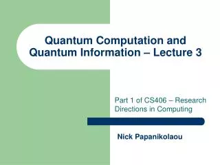
2. Content • Quantum information and computation – what for? • Quantum Bits and Algorithms • Implementations – Current Status • “Semi-Quantum” Computing • Conclusions

3. Quantum Information– what for? • First, quantum computers can crack some of the strongest cryptographic systems (e.g. RSA) • Second, they might be useful for various other things as well (simulating quantum systems etc.) • Quantum cryptography provides new solutions to some cryptographic problems • Quantum cryptography may become useful ALSO if (new) classical algorithms will crack RSA • Quantum Teleportation and quantum ECC can enlarge distance for secure quantum communication • Satellite quantum communication CREDIT: Science/AAAS

4. Quantum Computers– what for? • Quantum computers can crack RSA because they can factorize large numbers of n digits in polynomial time! O(n2 log n) • A “classical computer will have to work “sub-exponenital time” O(exp[(n log n)1/3]) CREDIT: Science/AAAS

5. Quantum Computers– what for? (2) • Quantum computers might be useful for various other things as well….. Mainly - simulating quantum systems: • Fully understanding the complicated electronic structures of molecules and molecular systems • Predicting reaction properties and dynamics • Designing well controlled state preparation • Analyzing protein folding • Understanding photosynthetic systems • HHL. Etc. Etc. Etc. • The HOPE is to have advantage already with 30-100 qubits CREDIT: Science/AAAS

6. Quantum Computers– what for? (3) • Quantum algorithms applied onto small “quantum computers” might be useful for various QUANTUM TASKS….. Mainly - manipulating quantum systems: • Algorithmic cooling of spins, for improving MRI/MRS/NMR/ESR is one of my team’s goals. • We collaborate on this topic with the one of the largest quantum computing centers – in Waterloo.Canada. • As said before: quantum ECC can enlarge distance for secure quantum communication CREDIT: Science/AAAS

7. D-Wave collaborations (Wikipedia) In 2011, Lockheed Martinsigned a contract with D-Wave Systems to realize the benefits based upon aquantum annealing processor applied to some of Lockheed's most challenging computation problems. The contract includes the purchase of a“128 qubit Quantum Computing System”. In 2013, a “512 qubit system” was sold to Google and NASA.

8. D-WAVE: Superconducting flux qubit MW Johnson et al.Nature473, 194-198 (May 2011) However, their “qubits” are highly limited. Similar Technology with less limited qubits reached 3-5 qubits, no more! So what is the TRUTH??

9. The Qubit In addition to the regular values {0,1} of a bit, and a probability distribution over these values, the Quantum bit can also be in a superposition www.cqed.org/IMG/jpg/compdoublemobilemz.jpg

10. The Qubit (2) A superposition state α|0› + β|1› Intereference (as in waves) scienceblogs.com http ://upload.wikimedia.org/wikipedia/commons/2/2c/Two_sources_interference.gif

11. The Qubit (2) A superposition state α|0› + β|1› Intereference (as in waves) scienceblogs.com http ://upload.wikimedia.org/wikipedia/commons/2/2c/Two_sources_interference.gif

12. The Qubit (2) A superposition state α|0› + β|1› … with |α|2+ |β|2 = 1 scienceblogs.com http ://upload.wikimedia.org/wikipedia/commons/2/2c/Two_sources_interference.gif

13. The Qubit (3) |+› = (1/√2) |0›+(1/√2) |1› Is a state of a particle in BOTH arms! But this is ALSO a state of a particle … in both arms |-› = (1/√2) |0›- (1/√2) |1› The amplitude 1/√2 means a probability of 1/2 to find the particle if we look for it, in one arm or another [In general: α|0› + β|1›  P(0)=|α|2and P(1)= |β|2]

14. The Qubit (4) The two arms meet - there is an interference This is so due to Linearity of quantum mechanics |0› → |+› = (1/√2) |0›+(1/√2) |1› |1› → |-› = (1/√2) |0›- (1/√2) |1› We get |+› = (1/√2) |0›+(1/√2) |1› → (1/√2) [(1/√2) |0›+(1/√2) |1›]+(1/√2) [(1/√2) |0› - (1/√2) |1›] = |0›“Constructive/Destructive Interference”

15. Two Qubits - Entanglement α|00› + β|11› brusselsjournal.com

16. Initialization (via Hadamard transformation) • Single qubit: |0› |+› = [|0›+|1›] / (1/√2) • Two qubits: |00› |++› = (1/2) [|00›+|01›+|10›+|11›] • For n qubits: |++ … +› = 1/(2n/2) ∑ i=0 |i› A superposition over all 2n possible values

17. Initialization (via Hadamard transformation) • Single qubit: |0› |+› = [|0›+|1›] / (1/√2) • Note: the Hadamard transformation is also responsible for the interference!!! |+›  |0›|-›|1›

18. n Qubits – parallel computing • Prepare a superposition • over 2n states • Run your algorithm • in parallel • Interference enhances the • probability of the desired solution • Peter Shor factorized large numbers (in principle) using Shor’s algorithm! • Several other problems in NP were also solved • Current quantum architecture reaches 13-14 qubits (NMR, ion trap); far from being practical… futuredocsblog.com

19. Will quantum computers factorize large numbers? • If ‘yes’ – this is a revolution in Computer Science • If ‘no’ – this is a revolution in Physics • So let’s assume it will… but maybe not so soon! • Can we predict when? futuredocsblog.com

20. Implementations • Ion trap (qubit is the ground-state vs excited-state of an electron attached to an ion; “many” ions in one trap) • NMR (qubit is the spin of a nuclei on a molecule; “many” spins on a molecule) • Josephson-Junction qubits (magnetic flux) • Optical qubits (photons) • Etc…

21. Example – ion trap Reached 14 (8) qubits Nobel Prize and Wolf Prize NIST sciencedaily.com

22. Reached 13 qubits Scalability problem Resolved via Algorithmic Cooling* Example - NMR tudelft.nl robert.nowotniak.com

23. Josephson Junctions (8-9 qubits, DWAVE 8**?) Q. Optics (6-7 qubits) Sufficient for some ECC Examples 3+4 The Australian Centre of Excellence for Quantum Computation and Communication Technology

24. Current status of fully-quantum computing • Despite the Nobel prize – we have no clue when ion traps will reach 25 qubits • Despite of 20M $ DWAVE computers already sold – we have no clue if JJ qubits are of any good; We do know (Shin, Smith Smolin, Vazirani; 2014) that there is probably no reason to believe that the DWAVE model is quantum**.

25. Current status of fully-quantum computing • Optmism – due to Moore’s Law for VLSI • Optimism – Semi QC

26. Limited QC Models:Semi-quantum computing • D-Wave’s AQC[???]; Other Q. Sim.? • One Clean Qubit * (closely related to NMR) • Linear Optics (closely related to Q. Optics) Three Extremely Important Questions: • What algorithms can the limited models run? [OCQ – Trace estimation; LO – boson sampling] • What kind of Quantumness/Entanglement is there? • Do they scale much easier/better than full QC?

27. (no) Conclusions • Zero conclusions about the future of full QC • Some optimism about semi-quantum computing • Many more questions than answers, both theoretically and experimentally Thanks

28. Appendix – DJ Algorithm • Initialization (1 slide) • Parallel computing (1 slide) • Deutsch’s Algorithm (6 slides): • Deutsch Problem (1 slide) • Classical solution (1 line) • Quantum solution (the remaining 5 slides)

29. Initialization( via Hadamrd Transformation) • Single qubit: |0› |+› = [|0›+|1›] / (1/√2) • Two qubits: |00› |++› = (1/2) [|00›+|01›+|10›+|11›] • For n qubits: |++ … +›= 1/(2n/2) ∑ i=0 |i› A superposition over all 2n possible values

30. Parallel Computing The quantum computer computes in parallel • If we know to classically apply U onto |00…0000›, onto |00…0001› etc, efficiently, we also immediately know how to apply it to that superposition |++…++++› • We get parallel computing over 2n values! • Interference yields the desired outcome!!

31. The first quantum algorithm(Deutsch, 1989) • We are given a black box calculating f(x), where x is a single bit, 0 or 1, and f(x) is also a single bit • We do not care what is f(0) and f(1), we only want to know if f(0)=f(1) [ is f constant? ] • Each call to the black box costs 1 Billion dollars, if we guess correctly the answer, we win 1.5 Billion dollars, if we fail we lose 2 Billions dollars! Can we become rich?

32. The first quantum algorithm(Deutsch, 1989) (2) • Classically we lose of course…. • With a quantum BOX – we may become rich! • We do not care for f(0) and f(1), we only need [f(0)==f(1)] ; We calculate this DIRECTLY!! • We shall use an additional (ancilla) qubit for keeping the result f(x): |x›|0› → |x›|f(x)› • We also plan that: |x›|1› → |x›|f(x)`› Did we become rich?

33. The first quantum algorithm(Deutsch, 1989) (3) • We plan the transformation: |x›|0› → |x›|f(x)› • We plan also: |x›|1› → |x›|f(x)`› • We prepare our ancilla: |-› = [|0›-|1›] / (1/√2) • We apply |x›|-› → |x›[|f(x)› - |f(x)`›] / (1/√2) • For x=0 we get: |0›[|f(0)› - |f(0)`›] / (1/√2) • For x=1 we get: |1›[|f(1)› - |f(1)`›] / (1/√2) Did we become rich?

34. The first quantum algorithm(Deutsch, 1989) (4) • For x=0 we get: |0›[|f(0)› - |f(0)`›] / (1/√2) • For x=1 we get: |1›[|f(1)› - |f(1)`›] / (1/√2) • But…. We prepare a superposition for x as well: [|0›+|1›] / (1/√2)… • And we get { |0›[|f(0)› - |f(0)`›] + |1›[|f(1)› - |f(1)`›] } / 2 Did we become rich?

35. The first quantum algorithm(Deutsch, 1989) (5) { |0›[|f(0)› - |f(0)`›] + |1›[|f(1)› - |f(1)`›] } / 2 • Case 1: f(0)=f(1)=b [ f is constant ]: { |0›[|b› - |b`›] + |1›[|b› - |b`›] } / 2 { [|0› + |1›] |b› - [|0› + |1›] |b’› } / 2 • Case 2: f(0)=c ; f(1)=c’: { |0›[|c› - |c`›] + |1›[|c’› - |c›] } / 2 { [|0› - |1›] |c› - [|0› - |1›] |c’› } / 2 Did we become rich?

36. The first quantum algorithm(Deutsch, 1989) (6) Let’s apply Hadamardtransformation onto the left qubit, and then measure it: • Case 1: f(0)=f(1)=b [ f is constant ]: { [|0› + |1›] |b› - [|0› + |1›] |b’› } / 2  [|0›|b› - |0› |b’›] / √2 = |0›[|b› - |b’›] / √2 • Case 2: f(0)=c ; f(1)=c’: { [|0› - |1›] |c› - [|0› - |1›] |c’› } / 2  [|1›|c› - |1› |c’›] / √2 = |1›[|c› - |c’›] / √2 We became rich!