Download
1 / 40
450 likes | 792 Views
Quantum Computation and Quantum Information – Lecture 3. Part 1 of CS406 – Research Directions in Computing. Nick Papanikolaou. Motivation. Quantum computers are built from wires and logic gates, just as classical computers are

E N D
Quantum Computation and Quantum Information – Lecture 3 Part 1 of CS406 – Research Directions in Computing Nick Papanikolaou
Motivation • Quantum computersare built from wires and logic gates, just as classical computers are • The potential of such devices stems from the ability to manipulate superpositions of states • Quantum algorithms solve problems which are not known to be solvable classically!
Lecture 3 Topics • Quantum logic gates • Simple quantum circuits • Quantum teleportation as a circuit • Deutsch’s quantum algorithm
Quantum vs. classical gates • The simplest boolean gate is NOT, with truth table: • Quantum gates have to be defined not only on the equivalents of 0 and 1, but on their superpositions too!
Quantum NOT gate: Linearity • Suppose we define a quantum NOT gate as follows: • The action of the quantum NOT gate on a superposition must then be: • All quantum operations are linear
The NOT Gate as a Matrix • Because all quantum operations have to be linear, we can represent the action of a quantum gate by a matrix • The quantum NOT, or Pauli-X gate, is written:
Quantum State Vectors • Remember that a quantum state is represented by a vector • Notation:
Quantum NOT • We can express the NOT operation on a general qubit as matrix multiplication:
Z Y H Other Single Qubit Gates • The Pauli-X gate works on only one qubit • Other common single qubit gates are: • Pauli-Z gate: • Pauli-Y gate: • Hadamard gate:
X Y Z H Summary of Simple Gates
Reversibility Requirement • All quantum operations have to bereversible • Boolean operations are not necessarily so • A reversible operation is always given by a unitary matrix, i.e. one for which:
The Controlled NOT Gate • The CNOT gate is the standard two-qubit quantum gate • It is defined like this:
The Controlled NOT Gate (2) • CNOT is a generalisation of the classical XOR: • The CNOT gate is drawn like this: “control qubit” “target qubit”
The Controlled NOT Gate (3) • The matrix corresponding to the CNOT gate is: • The CNOT together with the single qubit gates are universal for quantum computing
Quantum Circuits • Using the conventions for control and target qubits, we can build interesting circuits • Example: A Qubit Swap Circuit
Features of Quantum Circuits • No loops are allowed; quantum circuits are acyclic • Fan-in is not allowed: • Fan-out is not allowed:
Generalised Control Gate • Any quantum gate U can be converted into a controlled gate: One control qubit n target qubits U If the control qubit is “high,” U is applied to the targets. CNOT is the Controlled-X gate!
Quantum Measurement • Measurement in a quantum circuit is drawn as: M (classical bit representing outcome of measurement) M = 0 with prob. or M = 1 with prob. If then:
x x x x 0 y xÅy x A Qubit Cloning Circuit? • Using the XOR gate, it is possible to copy a classical bit: Can we build a quantum circuit that performs does this with qubits?
A Qubit Cloning Circuit? (2) OK here entangled!!
A Qubit Cloning Circuit? (3) It is impossible to clone a qubit! Also note that unwanted terms!
H The Bell State Circuit x y
H The Bell State Circuit By Example ?
Quantum Teleportation Circuit M1 H M2 XM2 ZM1
Quantum Teleportation Circuit (2) M1 H M2 XM2 ZM1 (|10>+|01>)
Quantum Teleportation Circuit (3) M1 H M2 XM2 ZM1
Quantum Teleportation Circuit (4) M1 H M2 XM2 ZM1 00, 01, 10 or 11
What have we achieved? • The teleportation process makes it possible to “reproduce” a qubit in a different location • But the original qubit is destroyed! • Next topic: Quantum Parallelism and Deutsch’s quantum algorithm
Quantum Parallelism • Quantum parallelism is that feature of quantum computers which makes it possible to evaluate a function f(x)on many different values ofxsimultaneously • We will look at an example of quantum parallelism now – how to compute f(0) and f(1) for some function f all in one go!
Quantum Circuits for Boolean Functions • It is known that, for any boolean function • it is possible to construct a quantum circuit Uf that computes it • Specifically, to each binary function f corresponds a quantum circuit: binary addition
x x y yÅf(x) Quantum Circuits for Boolean Functions (2) • What can this circuit Uf do? Example:
x x y yÅf(x) amazing! we’ve computed f(0) and f(1) at the same time! Quantum Circuits for Boolean Functions (3) • But what if the input is a superposition?
Quantum Parallelism Summary • So, a superposition of inputs will give a superposition of outputs! • We can perform many computations simultaneously • This is what makes famous quantum algorithms, such as Shor’s algorithm for factoring, or Grover’s algorithm for searching • Simple q. algorithm: Deutsch’s algorithm
Deutsch’s Algorithm • David Deutsch: famous British physicist • Deutsch’s algorithm allows us to compute, in only one step, the value of • To do this classically, you would have to: • compute f(0) • compute f(1) • add the two results • Remember:
x x y yÅf(x) H H H Circuit for Deutsch’s Algorithm
x x y yÅf(x) H H H Circuit for Deutsch’s Algorithm (2)
x x y yÅf(x) ...and so we have computed H H H Circuit for Deutsch’s Algorithm (3)
End of Lecture 3 • Congratulations! If you are still awake, you have learned something about: • quantum gates (X, Y, Z, H, CNOT) • quantum circuits (swapping, no-cloning problem) • teleportation • quantum parallelism • and Deutsch’s algorithm