Download
1 / 50
500 likes | 508 Views
MA/CSSE 474 Theory of Computation. More about Ambiguity Removal Normal Forms (Chomsky and Greibach) Pushdown Automata (PDA) Intro PDA examples. Your Questions?. HW10 or 11 problems Anything else. Previous class days' material Reading Assignments. Continue with Ambiguity Removal.

E N D
MA/CSSE 474 Theory of Computation More about Ambiguity Removal Normal Forms (Chomsky and Greibach) Pushdown Automata (PDA) Intro PDA examples
Your Questions? • HW10 or 11 problems • Anything else • Previous class days' material • Reading Assignments
Continue with Ambiguity Removal • Remove -rules (done last time) • Eliminate symmetric rules to control precedence and association • Deal with optional suffixes, such as if … else …
Recap: An Example G = {{S, T, A, B, C, a, b, c}, {a, b, c}, R, S), R = { SaTa TABC AaA | C BBb | C Cc | } removeEps(G: cfg) = 1. Let G = G. 2. Find the set N of nullable nonterminals in G. 3. Repeat until G contains no modifiable rules that haven’t been processed: Given the rule PQ, where QN, add the rule P if it is not already present and if and if P. 4. Delete from G all rules of the form X. 5. Return G. Recall: After this algorithm runs, L(G') = L(G) – {})
What If L? atmostoneEps(G: cfg) = 1. G = removeEps(G). 2. If SG is nullable then /* i. e., L(G) 2.1 Create in G a new start symbol S*. 2.2 Add to RG the two rules: S* S* SG. 3. Return G.
But There Can Still Be Ambiguity S* What about ()()() ? S* S SSS S (S) S ()
Eliminating Symmetric Recursive Rules S* S* S SSS S (S) S () Replace SSS with one of: SSS1 /* force branching to the left SS1S /* force branching to the right So we get: S* SSS1 S* S SS1 S1 (S) S1 ()
Eliminating Symmetric Recursive Rules S* S* S SSS1 SS1 S1 (S) S1 () S* S S S1 S S1 S1 ( ) ( ) ( )
Arithmetic Expressions EE + E EEE E (E) Eid Problem 1: Associativity E E EE EE EE EE id id id id id id
Arithmetic Expressions EE + E EEE E (E) Eid Problem 2: Precedence E E EE EE EE EE id id + id id id + id
Arithmetic Expressions - A Better Way EE + T ET TT * F TF F (E) F id
Ambiguous Attachment The dangling else problem: <stmt> ::= if <cond> then <stmt> <stmt> ::= if <cond> then <stmt> else <stmt> Consider: if cond1then if cond2then st1else st2
The Java Fix <Statement> ::= <IfThenStatement> | <IfThenElseStatement> | <IfThenElseStatementNoShortIf> <StatementNoShortIf> ::= <block> | <IfThenElseStatementNoShortIf> | … <IfThenStatement> ::= if ( <Expression> ) <Statement> <IfThenElseStatement> ::= if ( <Expression> ) <StatementNoShortIf> else <Statement> <IfThenElseStatementNoShortIf> ::= if ( <Expression> ) <StatementNoShortIf> else <StatementNoShortIf> <Statement> <IfThenElseStatement> if (cond) <StatementNoShortIf> else <Statement>
Going Too Far (removing Ambiguity) SNPVP NP the Nominal | Nominal | ProperNoun | NPPP Nominal N | Adjs N Ncat | girl | dogs | ball | chocolate | bat ProperNoun Chris | Fluffy AdjsAdj Adjs | Adj Adjyoung | older | smart VPV | V NP | VPPP Vlike | likes | thinks | hits PPPrep NP Prepwith ● Chris likes the girl with the cat. ● Chris shot the bear with a rifle.
Going Too Far ● Chris likes the girl with the cat. ● Chris shot the bear with a rifle. ● Chris shot the bear with a rifle.
Normal Forms A normal form F for a set C of data objects is a form, i.e., a set of syntactically valid objects, with the following two properties: ● For every element c of C, except possibly a finite set of special cases, there exists some element f of F such that f is equivalent to c with respect to some set of tasks. ● F is simpler than the original form in which the elements of C are written. By “simpler” we mean that at least some tasks are easier to perform on elements of F than they would be on elements of C.
Normal Form Examples ● Disjunctive normal form for database queries so that they can be entered in a query-by-example grid. ● Jordan normal form for a square matrix, in which the matrix is almost diagonal in the sense that its only non-zero entries lie on the diagonal and the superdiagonal. ● Various normal forms for grammars to support specific parsing techniques.
Normal Forms for Grammars Chomsky Normal Form, in which all rules are of one of the following two forms: ● Xa, where a, or ● XBC, where B and C are elements of V - . Advantages: ● Parsers can use binary trees. ● Bounds on length of derivations (what are they?) S A B A A B B aab B B bb
Normal Forms for Grammars Greibach Normal Form, in which all rules are of the following form: ● Xa, where a and (V - )*. Advantages: ● Bounds on length of derivations (what are they?) ● Greibach normal form grammars can easily be converted to pushdown automata with no - transitions. This is useful because such PDAs are guaranteed to halt.
Theorems: Normal Forms Exist Theorem: Given a CFG G, there exists an equivalent Chomsky normal form grammar GC such that: L(GC) = L(G) – {}. Proof: The proof is by construction. Theorem:Given a CFG G, there exists an equivalent Greibach normal form grammar GG such that: L(GG) = L(G) – {}. Proof: The proof is also by construction. Details of Chomsky conversion are complex but straightforward; I leave them for you to read in Chapter 11 and/or in the last 18 slides from today. Details of Greibach conversion are more complex but still straightforward; I leave them for you to read in Appendix D if you wish (not req'd).
The Price of Normal Forms EE + E E (E) Eid Converting to Chomsky normal form: EEE EPE ELE EE R Eid L ( R ) P + Conversion doesn’t change weak generative capacity but it may change strong generative capacity.
Comparing Regular and Context-Free Languages Regular Languages Context-Free Languages ● regular exprs. or ● regular grammars ● context-free grammars ● recognize ● parse (use a PDA)
Recognizing Context-Free Languages Two notions of recognition: (1) Say yes or no, just like with FSMs (2) Say yes or no, AND if yes, describe the structure a + b * c
Definition of a Pushdown Automaton M = (K, , , , s, A), where: K is a finite set of states is the input alphabet is the stack alphabet sK is the initial state AK is the set of accepting states, and is the transition relation. It is a finite subset of (K ( {}) *) (K*) state input string of state string of symbol symbols symbols or to pop to push from top on stack and are not necessarily disjoint
Definition of a Pushdown Automaton • A configuration of M is an element of • K* *. • The initial configuration of M is (s, w, ), where w is the input string.
Manipulating the Stack c will be written as cab a b If c1c2…cn is pushed onto the stack: c1 c2 cn c a b c1c2…cncab
Yields Let c be any element of {}, Let 1, 2 and be any elements of *, and Let w be any element of *. Then: (q1, cw, 1) ⊦M (q2, w, 2) iff ((q1, c, 1), (q2, 2)) . Let ⊦ M* be the reflexive, transitive closure of ⊦M. C1yields configuration C2 iff C1⊦M*C2
Computations A computation by M is a finite sequence of configurations C0, C1, …, Cn for some n 0 such that: ● C0 is an initial configuration, ● Cn is of the form (q, , ), for some state qKM and some string in *, and ● C0 ⊦MC1 ⊦MC2 ⊦M … ⊦MCn.
Nondeterminism If M is in some configuration (q1, s, ) it is possible that: ● contains exactly one transition that matches. ● contains more than one transition that matches. ● contains no transition that matches.
Accepting A computation C of M is an accepting computation iff: ● C = (s, w, ) ⊦M* (q, , ), and ● qA. Maccepts a string w iff at least one of its computations accepts. Other paths may: ● Read all the input and halt in a nonaccepting state, ● Read all the input and halt in an accepting state with the stack not empty, ● Loop forever and never finish reading the input, or ● Reach a dead end where no more input can be read. The language accepted byM, denoted L(M), is the set of all strings accepted by M.
Rejecting A computation C of M is a rejecting computation iff: ● C = (s, w, ) | ⊦M* (q, , ), ● C is not an accepting computation, and ● M has no moves that it can make from (q, , ). Mrejects a string w iff all of its computations reject. Note that it is possible that, on input w, M neither accepts nor rejects.
Details of CNF conversion • The remainder of the slides give an overview. • More details are in Chapter 11. • We will not cover these details in class.
Converting to a Normal Form 1. Apply some transformation to G to get rid of undesirable property 1. Show that the language generated by G is unchanged. 2. Apply another transformation to G to get rid of undesirable property 2. Show that the language generated by G is unchanged and that undesirable property 1 has not been reintroduced. 3. Continue until the grammar is in the desired form.
Rule Substitution XaYc Yb YZZ We can replace the X rule with the rules: Xabc XaZZc XaYcaZZc
Rule Substitution Theorem: Let G contain the rules: XY and Y1 | 2 | … | n , Replace XY by: X1, X2, …, Xn. The new grammar G' will be equivalent to G.
Details of Conversion to CNF • The rest of these slides summarize the CNF conversion • More detail is given in Chapter 11 of the textbook • We will not discuss this conversion process in class.
Rule Substitution Replace XY by: X1, X2, …, Xn. Proof: ● Every string in L(G) is also in L(G'): If XY is not used, then use same derivation. If it is used, then one derivation is: S … XYk … w Use this one instead: S … Xk … w ● Every string in L(G') is also in L(G): Every new rule can be simulated by old rules.
Convert to Chomsky Normal Form 1. Remove all -rules, using the algorithm removeEps. 2. Remove all unit productions (rules of the form AB). 3. Remove all rules whose right hand sides have length greater than 1 and include a terminal: (e.g., AaB or A BaC) 4. Remove all rules whose right hand sides have length greater than 2: (e.g., ABCDE)
Recap: Removing -Productions Remove all productions: (1) If there is a rule P Q and Q is nullable, Then: Add the rule P. (2) Delete all rules Q.
Removing -Productions Example: SaA AB | CDC B Ba CBD Db D
Unit Productions A unit production is a rule whose right-hand side consists of a single nonterminal symbol. Example: SX Y X A AB | a Bb YT TY | c
Removing Unit Productions removeUnits(G) = 1. Let G' = G. 2. Until no unit productions remain in G' do: 2.1 Choose some unit production X Y. 2.2 Remove it from G'. 2.3 Consider only rules that still remain. For every rule Y , where V*, do: Add to G' the rule X unless it is a rule that has already been removed once. 3. Return G'. After removing epsilon productions and unit productions, all rules whose right hand sides have length 1 are in Chomsky Normal Form.
Removing Unit Productions removeUnits(G) = 1. Let G' = G. 2. Until no unit productions remain in G' do: 2.1 Choose some unit production X Y. 2.2 Remove it from G'. 2.3 Consider only rules that still remain. For every rule Y , where V*, do: Add to G' the rule X unless it is a rule that has already been removed once. 3. Return G'. Example: SX Y X A AB | a Bb Y T T Y | c
Mixed Rules removeMixed(G) = 1. Let G = G. 2. Create a new nonterminal Ta for each terminal a in . 3. Modify each rule whose right-hand side has length greater than 1 and that contains a terminal symbol by substituting Ta for each occurrence of the terminal a. 4. Add to G, for each Ta, the rule Taa. 5. Return G. Example: Aa Aa B ABaC ABbC
Long Rules removeLong(G) = 1. Let G = G. 2. For each rule r of the form: AN1N2N3N4…Nn, n > 2 create new nonterminals M2, M3, … Mn-1. 3. Replace r with the rule AN1M2. 4. Add the rules: M2N2M3, M3N3M4, … Mn-1Nn-1Nn. 5. Return G. Example: ABCDEF
An Example SaACa AB | a BC | c CcC | removeEps returns: SaACa | aAa | aCa | aa AB | a BC | c CcC | c
An Example SaACa | aAa | aCa | aa AB | a BC | c CcC | c Next we apply removeUnits: Remove A B. Add A C | c. Remove BC. Add BcC (Bc, already there). Remove A C. Add A cC (Ac, already there). So removeUnits returns: SaACa | aAa | aCa | aa Aa | c | cC Bc | cC CcC | c
An Example SaACa | aAa | aCa | aa Aa | c | cC Bc | cC CcC | c Next we apply removeMixed, which returns: STaACTa | TaATa | TaCTa | TaTa Aa | c | TcC Bc | TcC CTcC | c Taa Tcc
An Example STaACTa | TaATa | TaCTa | TaTa Aa | c | TcC Bc | TcC CTcC | c Taa Tcc Finally, we apply removeLong, which returns: STaS1 STaS3 STaS4 STaTa S1AS2 S3ATaS4CTa S2CTaAa | c | TcC Bc | TcC CTcC | c Taa Tcc