Download
1 / 22
220 likes | 382 Views
4.4 Normal Forms. In this section, we shall introduce context-free grammars to two special forms, one is Chomsky normal form (CNF), the other is Greiback normal form (GNF). Definition 5: A CFG G = (V, T, P, S) is in Chomsky normal form if for each product of G is of the forms.

E N D
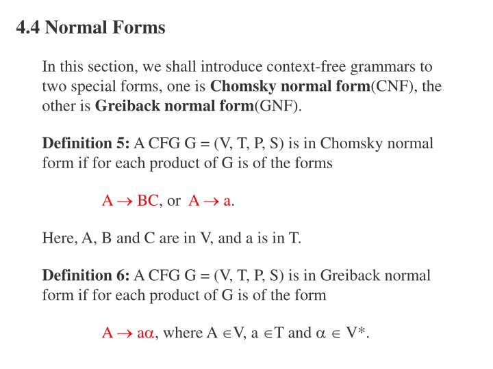
4.4 Normal Forms In this section, we shall introduce context-free grammars to two special forms, one is Chomsky normalform(CNF), the other is Greiback normalform(GNF). Definition 5: A CFG G = (V, T, P, S) is in Chomsky normal form if for each product of G is of the forms A BC, or A a. Here, A, B and C are in V, and a is in T. Definition 6: A CFG G = (V, T, P, S) is in Greiback normal form if for each product of G is of the form A a, where A V, a T and V*.
-productions An -production is of the form A . But, if the language L generated by a grammar G does not include , we can modify the grammar G to an equivalent grammar G’ so that there are no -productionsin G’. The algorithm to modify a grammar G to G’ is as follows. while ( there is a an -production A in G ) do remove the-production A from G If there is a production B xAy from G, then add a production B xy to G
Example 20: Consider the grammar G S 0T0 | 1T1 T 0T0 | 1T1 | Then L(G) = L = { x x R | x T*, and x }. We can modify the above grammar to a grammar without -productions as the following and generating the same language L. S 0T0 | 1T1 | 00 | 11 T 0T0 | 1T1 | 00 | 11 The above grammar is equivalent to the following grammar. S 0S0 | 1S1 | 00 | 11
Useless variables A is a useful variable if A * w for some w T*. For a CFG G, we can modify the grammar G to an equivalent grammar G’ so that there are no useless variables in G’. The algorithm to modify a grammar G to G’ is as follows. First, let the set S , flag TRUE while ( flag ) do // get useful variables flag FALSE If B T*in G, or B x 1A 1x 2A 2…x k A ky in G, where y, x i T* andA i S, i = 1,2, …, k, then S S {B}, flag TRUE The set V \ S is a set of useless variables.
Next, if there is a useless production B x 1A 1x 2A 2…x k A ky in G, where y, x i T* and one of B and A i, i = 1,2, …, k, is in V \ S, then remove the production B x 1A 1x 2A 2…x k A ky from G. The algorithm to remove useless variables and useless productions from the grammar G to get an equivalent grammar G’ without useless variables and useless productions.
Unit productions A unit production is of the form AB, where A and B are variables. A unit production basically is a redundant production. Therefore, we can eliminate the unit productions by the following method: For each unit production AB, remove the production from the grammar, and add the following productions: For each non-unit production Bw in G, add the production A w to G.
By the above algorithms, we are able to obtain the following theorem. Theorem 5 : For each CFL L without , there is a CFG G with no useless variables, -productionsor unit productions such that L(G) = L.
Theorem 6 : For each CFL L without , there is a CFG G in Chomsky normal form such that L(G) = L, i.e., each production in G is of the form A BC, or A a ,where A, B and C are in V, and a is in T. Proof : For each CFL L without , there is a CFG G with no useless variables, -productionsor unit productions such that L(G) = L. First step, for each productionA in G, if || = 1, then T. Otherwise, || > 1, say = X 1X 2…X k, k>1. IfX i , say i =1and X1= a, is a terminal and there is a production B a, then replace X 1 by B to get a new production A BX 2…X k , and remove the production A .
IfX i , say i =1and X 1 = a, is a terminal and there is no production Ba, then add a new variable C, and replace X 1 by C to get a new production A CX 2…X k , remove the production A and add a new production C a. After the first step, all productions are of the form either A a, or A , where || >1 and V+ Second step, for each production of the formA , where || >1, we know that V+. If || = 2, then we do not need to modify the production. If || > 2, say = X 1X 2…X k, k>2, then we need to introduce new variables Y 1 ,Y 2 ,… , Y k-2, and add the new productions as follows.
A X 1Y 1 Y 1X 2Y 2 Y iX i+1Y i+1, i = 1, 2, …, k3, Y k-3X k-2Y k-2 Y k-2X k-1X k Therefore, we can modify the grammar to a new equivalent grammar in Chomsky normal form.
Theorem 7 : For each CFL L without , there is a CFG G in Greiback normal form such that L(G) = L. Proof : For each CFL L without , there is a CFG G’’ with no useless variables, -productionsor unit productions such that L(G’’) = L. By theorem 6, there is a CFG G’=(V’, T, P’, S’) in Chomsky normal form such that L(G’) = L(G’’) = L. Rewrite the k variables in V’ with indices 1, 2, …, k. Let it be V = {A 1, A 2, …, A k} and the start variable is A 1.
First step, modify the productions into the forms A ia, where a T and V*, or A iA j , where j >i To achieve the result, we start from A 1. If there is a production A 1a, where a T and V*, then we keep the production. If there is a production A 1A 1, then apply theorem 4 in section 4.2 to revise the left recursive production to a right recursive production until there is no A 1recursive production. Next we revise the A 2 productions until A k. A possible algorithm for this step is as follows.
for i=1 to k do for j=1 to i 1 do for each production A i A j do for each production A j do add production A i remove production A i A j for each production A i A i do add productions B i and B i B i remove productions A i A i for each production A i , where does not begin with A i do add production A i B i
After the first step, the productions are of the forms: A ia, where a T and V*, A iA j , where k j > i, or B i, where ( V{B 1, B 2,…, B i1} )*. The A k production must be of the form A ka, where a T and V*, The B i production must be of the form B iA j, where (V {B 1, B 2,…, B i1}) *, or B ia, where a T and (V {B 1, B 2,…, B i1}) *,
Second step, modify each A i production into the forms A ia, where a T and V*. To achieve the result, we start from A k1to modify the A k1productions so that the right side of the production starting with a terminal. Then proceed the same process until A 1. A possible algorithm for this step is as follows. for i=k 1 to 1 do for j=k to i +1 do for each production A i A j do for each production A j do add production A i remove production A i A j
Third step, modify each B i production into the forms B ia, where a T and V*. A possible algorithm for this step is as follows. for i=1 to k do for each production B i A j do for each production A j do add production A j remove production B i A j
Example 21: Consider the grammar G S 0S0 | 1S1 | 00 | 11 An equivalent CFG in GNF is S 0SZ | 1SY | 0Z | 1Y Y 1 Z 0 An equivalent CFG in CNF is S ZX | YW | ZZ | YY X SZ W SY Y 1 Z 0
Example 22: Convert the grammar G in CNF to a grammar in GNF : A 1A 1 A 2| A 3 A 1 A 2A 1 A 3| 0 A 3 A 1 A 2| 1 Solution: First stage: Step 1: Introduce variable B 1 to modify the productions A 1A 1 A 2| A 3 A 1 to the following productions: A 1 A 3 A 1 | A 3 A 1 B 1 B 1 A 2 | A 2 B 1
Step 2: Modify the productions A 2A 1 A 3 | 0 to the following productions: A 2 A 3 A 1 A 3 | A 3 A 1 B 1 A 3 | 0 Step 3: Modify the productions A 3 A 1 A 2| 1to the following productions: A 3 A 3 A 1 A 2| A 3 A 1 B 1 A 2| 1 Step 4: Introduce variable B 3 to modify the productions A 3A 3 A 1 A 2 | A 3 A 1 B 1 A 2| 1 to the following production: A 3 1 | 1B 3 B 3 A 1 A 2 B 3| A 1 B 1 A 2 B 3 | A 1 A 2 | A 1 B 1 A 2
After the first stage we have the following productions: A 1 A 3 A 1 | A 3 A 1 B 1 B 1 A 2 | A 2 B 1 A 2 A 3 A 1 A 3 | A 3 A 1 B 1 A 3 | 0 A 3 1 | 1B 3 B 3 A 1 A 2 B 3| A 1 B 1 A 2 B 3 | A 1 A 2 | A 1 B 1 A 2
Second stage: Step 5: By A 3 productions A 3 1 | 1B 3 , modify the A 2 productions to the following productions: A 2 1A 1 A 3 | 1 B 3 A 1 A 3 | 1A 1 B 1 A 3 | 1 B 3 A 1 B 1 A 3 | 0 Step 6: Modify the A 1 productions to the following productions: A 1 1A 1 | 1 B 3 A 1 | 1A 1 B 1 | 1 B 3 A 1 B 1 After the second stage, we have the following productions: A 1 1A 1 | 1 B 3 A 1 | 1A 1 B 1 | 1 B 3 A 1 B 1 A 2 1A 1 A 3 | 1 B 3 A 1 A 3 | 1A 1 B 1 A 3 | 1 B 3 A 1 B 1 A 3 | 0 A 3 1 | 1B 3 B 1 A 2 | A 2 B 1 B 3 A 1 A 2 B 3| A 1 B 1 A 2 B 3 | A 1 A 2 | A 1 B 1 A 2
Third stage: Step 7: Modify the Bproductions to the following productions: A 1 1A 1 | 1 B 3 A 1 | 1A 1 B 1 | 1 B 3 A 1 B 1 A 2 1A 1 A 3 | 1 B 3 A 1 A 3 | 1A 1 B 1 A 3 | 1 B 3 A 1 B 1 A 3 | 0 A 3 1 | 1B 3 B 1 1A 1 A 3 | 1 B 3 A 1 A 3 | 1A 1 B 1 A 3 | 1 B 3 A 1 B 1 A 3 | 0 B 1 1A1A3B1 | 1B3A1A3B1 | 1A1B1A3B1 | 1B 3A1B1A3B1 | 0B1 B 3 1A 1A 2B 3 | 1B 3A 1A 2B 3 | 1A 1B 1A 2B 3 | 1B 3A 1B 1A 2B 3 B3 1A1B1A2B3 |1B3A1B1A2B3 |1A1B1B1A2B3 |1B3A1B1B1A2B3 B 3 1A 1 A 2 | 1 B 3 A 1 A 2 | 1A 1 B 1 A 2 | 1 B 3 A 1 B 1 A 2 B 3 1A1B1A2 | 1B3A1B1A2 | 1A1B1B1A2 | 1B3A1B1B1A 2