Download
1 / 11
110 likes | 121 Views
Chapter 12 Simple Linear Regression and Correlation. Simple Linear Regression Model Y = 1 x + 0 + Random Error: is N(0, 2 ) RV.

E N D
Simple Linear Regression ModelY = 1x + 0 + Random Error: is N(0, 2) RV
Least Squares Estimates of 0, 1, and 2Slope 1 = SXY = xiyi – (xi)(yi) / n SXX (x2i) – (xi)2 / nIntercept 0 = y - 1x s2 = SSE = (y2i) - 0yi - 1xiyi n – 2 n – 2
Example: Regression AnalysisYou have collected data on construction of standard cabinets for capacity planning issues. The following data shows the time (y) in hours for a 2-man team to complete an assigned number of cabinets (x) before going to another job of different design.NumberTime (hours) Number Time (hours) 1 0.9 2 1.8 4 3.0 4 2.4 7 4.2 5 3.2 3 2.5 3 2.0 Assuming that the linear regression model is valid, obtain the least square estimate of the true regression line. Marketing has just learned of your linear regression model. For costing purposes, marketing wants to know the probability that it will take more than 3 hours to complete 4 cabinets?
Sample Correlation Coefficientr = SXYSXX SYYr = xiyi – [(xi)(yi) / n](x2i)–[(xi)2 / n](y2i)–[(yi)2 / n]Relationship between variables:Rule Of Thumb: Strong if .8 r 1 Weak if 0 r .5
Example Correlation CoefficientIn studying the effect of pollution on a lake, researchers take measurements of the nitrate concentration of the water. An older manual method has been used to monitor this variable. However, a new automated method has been devised. If a high positive correlation exists between the measurements taken by using the two methods, then the automated method will be put into routine use. The data obtained on the nitrate concentration in micrograms of nitrate per liter of water follows:x (manual) y (auto) x (manual) y (auto) 25 30 40 80 120 150 75 80 150 200 300 350 270 240 400 320 450 470 575 583
Coefficient of Determinationr2 = 1 –SSE = 1 –(yi – yi)2 SST (yi – y)2Amount of variability in the data accounted for by the regression model.(yi – y)2 = (y2i) – (yi)2 / n
Example: Coefficient of DeterminationData is collected for (3) different cities where the commuting time (y) is plotted against commuting distance (x). The data summary follows:City 1 City 2 City 3SXX 17.5 1270.8333 1270.8333SXY 29.5 2722.5 1431.66671 1.685714 2.142295 1.1265570 13.666672 7.868852 3.196729SST 114.83 5897.5 1627.33SSE 65.1 65.1 14.48 (n = 6)Based on values of s and r2, for which city would a simple linear regression model be most effective?
Prediction of Y-valuesMean Value of Y*: E(Y*) = 0 + 1x*Variance of Y*: V(Y*) = s2 + s21 + (x* - x)2 n SXXSXX = (x2i) – [(xi)2 / n]
Example: Prediction of Y-valuesA study on infestation of crops by insects includes a report on the age (x) of a cotton plant (days) and the percent damaged area (y). Consider the accompanying data for 12 observations:xi= 246 yi= 572 (x-range 9 to 33)x2i= 5,742 y2i= 35,634 xiyi = 14,022Predict the percentage of damaged area when the age is 20 days. Supply an estimated standard deviation with your answer.
Simple Linear Regression AnalysisRegression analysis can be used for quantitative forecasting. We use our knowledge about the relationship between a dependent and independent variable to estimate the future values of the dependent variable. If the underlying data form a time series, the independent variable is time periods.Example: Your company produces electronic motors for power-actuated valves for the construction industry. Your plant has operated at near capacity for over a year. You feel that the growth in sales will continue and you want to develop a long-range forecast to be used to plan facility requirements for the next two years. Sales records for the past ten years have been accumulated.Year Annual Sales Year Annual Sales (unitsx1,000) 1 1,000 6 2,000 2 1,300 7 2,200 3 1,800 8 2,600 4 2,000 9 2,900 5 2,000 10 3,200Develop a long-range forecast using the least squares principles to assist in planning the facilities for the next (2) years. Provide expected values, standard deviations, & coefficients of correlation and determination.