Download
1 / 63
670 likes | 1.03k Views
Chapter 12. Simple Linear Regression and Correlation. 12.1 The Simple Linear Regression Model 12.2 Fitting the Regression Line 12.3 Inferences on the Slope Parameter β 1 12.4 Inferences on the Regression Line 12.5 Prediction Intervals for Future Response Values

E N D
Chapter 12. Simple Linear Regression and Correlation 12.1 The Simple Linear Regression Model 12.2 Fitting the Regression Line 12.3 Inferences on the Slope Parameter β1 12.4 Inferences on the Regression Line 12.5 Prediction Intervals for Future Response Values 12.6 The Analysis of Variance Table 12.7 Residual Analysis 12.8 Variable Transformations 12.9 Correlation Analysis 12.10 Supplementary Problems
12.1 The Simple Linear Regression Model12.1.1 Model Definition and Assumptions(1/5) • With the simple linear regression model yi=β0+β1xi+εi the observed value of the dependent variable yi is composed of a linear function β0+β1xi of the explanatory variable xi, together with an error termεi. The error terms ε1,…,εn are generally taken to be independent observations from a N(0,σ2) distribution, for some error varianceσ2. This implies that the values y1,…,yn are observations from the independent random variables Yi~ N (β0+β1xi, σ2) as illustrated in Figure 12.1
12.1.1 Model Definition and Assumptions(3/5) • The parameter β0 is known as the intercept parameter, and the parameter β0 is known as the intercept parameter, and the parameter β1 is known as the slope parameter. A third unknown parameter, the error variance σ2, can also be estimated from the data set. As illustrated in Figure 12.2, the data values (xi , yi ) lie closer to the line y= β0+β1x as the error variance σ2 decreases.
12.1.1 Model Definition and Assumptions(4/5) • The slope parameterβ1 is of particular interest since it indicates how the expected value of the dependent variable depends upon the explanatory variable x, as shown in Figure 12.3 • The data set shown in Figure 12.4 exhibits a quadratic (or at least nonlinear) relationship between the two variables, and it would make no sense to fit a straight line to the data set.
12.1.1 Model Definition and Assumptions(5/5) • Simple Linear Regression Model The simple linear regression model yi = β0 + β1xi + εi fits a straight line through a set of paired data observations (x1,y1),…,(xn, yn). The error terms ε1,…,εn are taken to be independent observations from a N(0,σ2) distribution. The three unknown parameters, the intercept parameterβ0 , the slope parameterβ1, and the error varianceσ2, are estimated from the data set.
12.1.2 Examples(1/2) • Example 67 : Car Plant Electricity Usage The manager of a car plant wishes to investigate how the plant’s electricity usage depends upon the plant’s production. The linear model will allow a month’s electrical usage to be estimated as a function of the month’s pro- duction.
12.2 Fitting the Regression Line12.2.1 Parameter Estimation(1/4)
12.2.2 Examples(1/5) • Example 67 : Car Plant Electricity Usage
12.2.2 Examples(2/5) Fig. 12.16
12.2.2 Examples(4/5) Fig. 12.17
12.3 Inferences on the Slope Parameter β112.3.1 Inference Procedures Inferences on the Slope Parameter β1
12.3 Inferences on the Slope Parameter β112.3.1 Inference Procedures Inferences on the Slope Parameter β1
Slki Lab. 12.3.1 Inference Procedures
12.3.1 Inference Procedures • An interesting point to notice is that for a fixed value of the error variance σ2, the variance of the slope parameter estimate decreases as the value of SXX increases. This happens as the values of the explanatory variable xi become more spread out, as illustrated in Figure 12.30. This result is intuitively reasonable since a greater spread in the values xi provides a greater “leverage” for fitting the regression line, and therefore the slope parameter estimate should be more accurate. Fig. 12.21
12.3.2 Examples(1/2) • Example 67 : Car Plant Electricity Usage
12.4 Inferences on the Regression Line12.4.1 Inference Procedures Inferences on the Expected Value of the Dependent Variable
12.4 Inferences on the Regression Line12.4.1 Inference Procedures Inferences on the Expected Value of the Dependent Variable
12.4 Inferences on the Regression Line12.4.1 Inference Procedures Inferences on the Expected Value of the Dependent Variable
12.4 Inferences on the Regression Line12.4.1 Inference Procedures Inferences on the Expected Value of the Dependent Variable
12.4.2 Examples(1/2) • Example 67 : Car Plant Electricity Usage
12.4.2 Examples(2/2) Fig. 12.23
12.5 Prediction Intervals for Future Response Values12.5.1 Inference Procedures(1/2) • Prediction Intervals for Future Response Values
12.5.2 Examples(1/2) • Example 67 : Car Plant Electricity Usage
12.5.2 Examples(2/2) Fig. 12.26
12.6 The Analysis of Variance Table12.6.1 Sum of Squares Decomposition(1/5) Fig. 12.29
12.6.1 Sum of Squares Decomposition(2/5) Fig. 12.30
12.6.1 Sum of Squares Decomposition(3/5) Consider the null hypothesis test F I G U R E 12.31 Analysis of variance table for simple linear regression analysis
12.6.1 Sum of Squares Decomposition(4/5) Fig. 12.32
12.6.1 Sum of Squares Decomposition(5/5) Coefficient of Determination R2
12.6.2 Examples(1/1) • Example 67 : Car Plant Electricity Usage
12.7 Residual Analysis12.7.1 Residual Analysis Methods(1/7) • The residuals are defined to be so that they are the differences between the observed values of the dependent variable and the corresponding fitted values . • A property of the residuals • Residual analysis can be used to • Identify data points that are outliers, • Check whether the fitted model is appropriate, • Check whether the error variance is constant, and • Check whether the error terms are normally distributed.
12.7.1 Residual Analysis Methods(2/7) • A nice random scatter plot such as the one in Figure 12.38 ⇒ there are no indications of any problems with the regression analysis • Any patterns in the residual plot or any residuals with a large absolute value alert the experimenter to possible problems with the fitted regression model. Fig. 12.38
12.7.1 Residual Analysis Methods(3/7) • A data point (xi, yi ) can be considered to be an outlier if it does not appear to predict well by the fitted model. • Residuals of outliers have a large absolute value, as indicated in Figure 12.39. Note in the figure that is used instead of • [For your interest only] Fig. 12.39
12.7.1 Residual Analysis Methods(4/7) • If the residual plot shows positive and negative residuals grouped together as in Figure 12.40, then a linear model is not appropriate. As Figure 12.40 indicates, a nonlinear model is needed for such a data set. Fig. 12.40
12.7.1 Residual Analysis Methods(5/7) • If the residual plot shows a “funnel shape” as in Figure 12.41, so that the size of the residuals depends upon the value of the explanatory variable x, then the assumption of a constant error variance σ2 is not valid. Fig. 12.41
12.7.1 Residual Analysis Methods(6/7) • A normal probability plot ( a normal score plot) of the residuals • Check whether the error terms εi appear to be normally distributed. • The normal score of the i th smallest residual • The main body of the points in a normal probability plot lie approximately on a straight line as in Figure 12.42 is reasonable • The form such as in Figure 12.43 indicates that the distribution is not normal
12.7.1 Residual Analysis Methods(7/7) Fig. 12.42 Fig. 12.43
12.7.2 Examples(1/2) Fig. 12.44 • Example : Nile River Flowrate