Download
1 / 36
360 likes | 567 Views
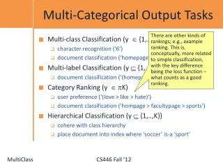
Multi-Categorical Output Tasks. There are other kinds of rankings; e.g., example ranking. This is, conceptually, more related to simple classification, with the key difference being the loss function – what counts as a good ranking. Multi-class Classification (y {1,...,K})

E N D
Multi-Categorical Output Tasks There are other kinds of rankings; e.g., example ranking. This is, conceptually, more related to simple classification, with the key difference being the loss function – what counts as a good ranking. • Multi-class Classification (y {1,...,K}) • character recognition (‘6’) • document classification (‘homepage’) • Multi-label Classification (y {1,...,K}) • document classification (‘(homepage,facultypage)’) • Category Ranking (y K) • user preference (‘(love > like > hate)’) • document classification (‘hompage > facultypage > sports’) • Hierarchical Classification (y {1,..,K}) • cohere with class hierarchy • place document into index where ‘soccer’ is-a ‘sport’
One-Vs-All • Assumption: Each class can be separated from the rest using a binary classifier in the hypothesis space. • Learning: Decomposed to learning k independent binary classifiers, one corresponding to each class. • An example (x,y) is considered positive for class y and negative to all others. • Assume m examples, k class labels. For simplicity, say, m/k in each. • classifier fi: m/k (+) and (k-1)m/k (-) • Decision: Winner Takes All (WTA): • f(x) = argmaxi fi (x) = argmaxi vi x
Solving MultiClass with binary learning • MultiClass classifier • Function f : Rd {1,2,3,...,k} • Decompose into binary problems • Not always possible to learn • No theoretical justification • (unless the problem is easy)
Learning via One-Versus-All (OvA) Assumption • Find vr,vb,vg,vyRn such that • vr.x > 0 iff y = red • vb.x > 0 iff y = blue • vg.x > 0 iff y = green • vy.x > 0 iff y = yellow • Classification: f(x)= argmaxivi x H = Rkn Real Problem
All-Vs-All • Assumption: There is a separation between every pair of classes using a binary classifier in the hypothesis space. • Learning: Decomposed to learning [k choose 2] ~ k2independent binary classifiers, one corresponding to each class. • An example (x,y) is considered positive for class y and negative to all others. • Assume m examples, k class labels. For simplicity, say, m/k in each. • Classifier fij: m/k (+) and m/k (-) • Decision: Winner Decision procedure is more involved since output of binary classifier may not cohere. Options: • Majority: classify example x to take label iif i wins on it more often that j (j=1,…k) • Use real valued output (or: interpret output as probabilities) • Tournament: start with n/2 pairs; continue with winners .
H = Rkkn How to classify? Learning via All-Verses-All (AvA) Assumption • Find vrb,vrg,vry,vbg,vby,vgyRd such that • vrb.x > 0 if y = red < 0 if y = blue • vrg.x > 0 if y = red < 0 if y = green • ... (for all pairs) Individual Classifiers Decision Regions
Tree Majority Vote 1 red, 2 yellow, 2 green ? Tournament Classifying with AvA All are post-learning and might cause weird stuff
Error Correcting Codes Decomposition • 1-vs-all uses k classifiers for k labels; can you use only log2 k? • Reduce the multi-class classification to random binary problems. • Choose a “code word” for each label. • Rows: An encoding of each class (k rows) • Columns: L dichotomies of the data, each corresponds to a new classification problem • Extreme cases: • 1-vs-all: k rows, k columns • K rows log2 k columns • Each training example is mapped to one example per column • (x,3) {(x,P1), +; (x,P2), -; (x,P3), -; (x,P4), +} • To classify a new example x: • Evaluate hypothesis on the 4 binaryproblems {(x,P1) , (x,P2), (x,P3), (x,P4),} • Choose label that is most consistent with the results. • Nice theoretical results as a function of the performance of the Pi s (depending on code & size) • Potential Problems?
Problems with Decompositions • Learning optimizes over local metrics • Poor global performance • What is the metric? • We don’t care about the performance of the local classifiers • Poor decomposition poor performance • Difficult local problems • Irrelevant local problems • Especially true for Error Correcting Output Codes • Another (class of) decomposition • Difficulty: how to make sure that the resulting problems are separable. • Efficiency: e.g., All vs. All vs. One vs. All • Former has advantage when working with the dual space. • Not clear how to generalize multi-class to problems with a very large # of output.
A sequential model for multiclass classification • A practical approach: towards a pipeline model • As before: relies on a decomposition of the Y space • This time, a hierarchical decomposition • (but sometimes the X space is also decomposed) • Goal: Deal with large Y space. • Problem: the performance of a multiclass classifier goes down with the growth in the number of labels.
A sequential model for multiclass classification • Assume Y = {1, 2, …k } • In the course of classifying we build a collection of subsets: Yd …½Y2µ Y1µY0 =Y • Idea: sequentially, learn fi: X !Yi-1 (i=1,…d) • fi is used to restrict the set of labels; • In the next step we deal only with labels in Yi • fi outputs a probability distribution over labels in Yi-1: Pi = (pi ( y1 | x), ….pi ( ym| x)) • Define: Yi = {y 2 Y | pi ( y |x) > i} (other decision rules possible) • Now we need to deal with a smaller set of labels.
Example: Question Classification • A common first step in Question Answering determines the type of the desired answer: Examples: • 1. What is bipolar disorder? • definition or disease/medicine • 2. What do bats eat? • Food, plant or animal • 3. What is the PH scale? • Could be a numeric value or a definition
Example: A hierarchical QC Classifier • The initial confusion set of any question is C0 (coarse classes) • The coarse classifier determines a set of preferred labels, C1µC0, with |C1|<5 (tunable) • Each coarse label is expanded to a set of fine labels using the fixed hierarchy to yield C2 • This process continues now on the fine labels, to yield C3µC2 • Output C1, C3(or continue)
1 Vs All: Learning Architecture • k label nodes; n input features, nk weights. • Evaluation: Winner Take All • Training: Each set of n weights, corresponding to the i-th label is trained independently given its performance on example x, and independently of the performance of label j on x. • However, this architecture allows multiple learning algorithm; e.g., see the implementation in the SNoWMulti-class Classifier Targets (each an LTU) Weighted edges (weight vectors) Features
Recall: Winnow’s Extensions Positive w+ Negative w- • Winnow learns monotone Boolean functions • We extended to general Boolean functions via • “Balanced Winnow” • 2 weights per variable; • Decision: using the “effective weight”, the difference between w+ and w- • This is equivalent to the Winner take all decision • Learning: In principle, it is possible to use the 1-vs-all rule and update each set of n weights separately, but we suggested the “balanced” Update rule that takes into account how both sets of n weights predict on example x
An Intuition: Balanced Winnow • In most multi-class classifiers you have a target node that represents positive examples and target node that represents negative examples. • Typically, we train each node separately (mine/not-mine example). • Rather, given an example we could say: this is more a + example than a – example. • We compared the activation of the different target nodes (classifiers) on a given example. (This example is more class + than class-) • Can this be generalized to the case of k labels, k >2?
Constraint Classification • The examples we give the learner are pairs (x,y), y 2 {1,…k} • The “black box learner” we described seems like it is a function of only x but, actually, we made use of the labels y • How is y being used? • y decides what to do with the example x; that is, which of the k classifiers should take the example as a positive example (making it a negative to all the others). • How do we make decisions: • Let: fy(x) = wyT¢ x • Then, we predict using: y* = argmaxy=1,…kfy(x) • Equivalently, we can say that we predict as follows: • Predict yiff • 8 y’ 2 {1,…k}, y’:=y (wyT– wy’T) ¢ x ¸ 0 (**) • So far, we did not say how we learn the k weight vectors wy (y = 1,…k)
Linear Separability for Multiclass • We are learning kn-dimensional weight vectors, so we can concatenate the k weight vectors into w= (w1, w2,…wk) 2Rnk • Key Construction: (Kesler Construction; Zimak’s Constraint Classification) • We will represent each example (x,y), as an nk-dimensional vector, xywith x embedded in the y-th part of it (y=1,2,…k) and the other coordinates are 0. • E.g., xy= (0,x,0,0) Rkn(here k=4, y=2) • Now we can understand the decision • Predict yiff 8y’ 2 {1,…k}, y’:=y (wyT– wy’T) ¢ x ¸ 0 (**) • In the nk-dimensional space. • Predict yiff 8y’ 2 {1,…k}, y’:=y wT¢(xy – xy’) wT¢xyy’¸ 0 • Conclusion: The set (xyy’, + ) (xy – xy’ , +) is linearly separable from the set (-xyy’ , - ) using the linear separator w 2Rkn’ • We solved the voroni diagram challenge.
2>4 2>1 2>3 2>1 2>3 2>4 Details: Kesler Construction & Multi-Class Separability If (x,i) was a given n-dimensional example (that is, x has is labeled i, then xij, 8 j=1,…k, j:= i, are positive examples in the nk-dimensional space. –xijare negative examples. • Transform Examples i>j fi(x) - fj(x) > 0 wi x - wj x > 0 WXi - WXj > 0 W (Xi - Xj) > 0 WXij > 0 Xi = (0,x,0,0) Rkd Xj = (0,0,0,x) Rkd Xij = Xi -Xj = (0,x,0,-x) W = (w1,w2,w3,w4) Rkd
Kesler’s Construction (1) • y = argmaxi=(r,b,g,y)wi.x • wi, xRn • Find wr,wb,wg,wyRn such that • wr.x> wb.x • wr.x> wg.x • wr.x> wy.x H = Rkn
x -x -x x Kesler’s Construction (2) • Let w= (wr,wb,wg,wy) Rkn • Let 0n, be the n-dim zero vector • wr.x> wb.x w.(x,-x,0n,0n) > 0 w.(-x,x,0n,0n) < 0 • wr.x> wg.x w.(x,0n,-x,0n) > 0 w.(-x,0n,x,0n) < 0 • wr.x> wy.x w.(x,0n,0n,-x) > 0 w.(-x,0n,0n ,x) < 0
x -x Kesler’s Construction (3) • Let • w= (w1, ..., wk) Rn x ... x Rn= Rkn • xij = (0(i-1)n, x, 0(k-i)n) – (0(j-1)n, –x, 0(k-j)n) Rkn • Given (x, y) Rn x {1,...,k} • For all j y • Add to P+(x,y), (xyj, 1) • Add to P-(x,y), (–xyj, -1) • P+(x,y) has k-1 positive examples (Rkn) • P-(x,y) has k-1 negative examples (Rkn)
Learning via Kesler’s Construction • Given (x1, y1), ..., (xN, yN) Rn x {1,...,k} • Create • P+ = P+(xi,yi) • P– = P–(xi,yi) • Find w= (w1, ..., wk) Rkn, such that • w.xseparates P+ from P– • One can use any algorithm in this space: Perceptron, Winnow, etc. • To understand how to update the weight vector in the n-dimensional space, we note that • wT¢xyy’¸ 0 (in the nk-dimensional space) • is equivalent to: • (wyT– wy’T) ¢ x ¸ 0 (in the n-dimensional space)
Learning via Kesler Construction (2) • A perceptron update rule applied in the nk-dimensional space due to a mistake in wT¢xij¸ 0 • Or, equivalently to (wiT– wjT) ¢ x ¸ 0 (in the n-dimensional space) • Implies the following update: • Given example (x,i) (example x 2Rn, labeled i) • 8 (i,j), i,j = 1,…k, i:= j (***) • If (wiT- wjT) ¢ x < 0 (mistaken prediction; equivalent to wT¢xij¸ 0 ) • wi wi +x (promotion) andwj wj – x (demotion) • Note that this is a generalization of balanced Winnow rule. • Note that we promote wiand demote k-1 weight vectors wj
Conservative update • The general scheme suggests: • Given example (x,i) (example x 2Rn, labeled i) • 8 (i,j), i,j = 1,…k, i:= j (***) • If (wiT- wjT) ¢ x < 0 (mistaken prediction; equivalent to wT¢xij¸ 0 ) • wi wi +x (promotion) andwj wj – x (demotion) • Promote wiand demote k-1 weight vectors wj • A conservative update: (SNoW’s implementation): • In case of a mistake: only the weights corresponding to the target node i and that closest node j are updated. • Let: j* = argminj=1,…k(wiT- wjT) ¢ x • If (wiT– wj*T ) ¢ x < 0 (mistaken prediction) • wi wi+x (promotion) andwj* wj*– x (demotion) • Other weight vectors are not being updated.
Significance • The hypothesis learned above is more expressive than when the OvA assumption is used. • Any linear learning algorithm can be used, and algorithmic-specific properties are maintained (e.g., attribute efficiency if using winnow. • E.g., the multiclass support vector machine can be implemented by learning a hyperplane to separate P(S) with maximal margin. • As a byproduct of the linear separability observation, we get a natural notion of a margin in the multi-class case, inherited from the binary separability in the nk-dimensional space. • Given example xij2Rnk, margin(xij,w) = minijwT¢xij • Consequently, given x2Rn, labeled i margin(x,w) = minj (wiT- wjT) ¢ x
Constraint Classification • The scheme presented can be generalized to provide a uniform view for multiple types of problems: multi-class, multi-label, category-ranking • Reduces learning to a single binary learning task • Captures theoretical properties of binary algorithm • Experimentally verified • Naturally extends Perceptron, SVM, etc... • It is called “constraint classification” since it does it all by representing labels as a set of constraints or preferences among output labels.
Multi-category to Constraint Classification Just like in the multiclass we learn one wi2Rn for each label, the same is done for multi-label and ranking. The weight vectors are updated according with the requirements from y 2Sk • The unified formulation is clear from the following examples: • Multiclass • (x, A) (x, (A>B, A>C, A>D) ) • Multilabel • (x, (A, B)) (x, ( (A>C, A>D, B>C, B>D) ) • Label Ranking • (x, (5>4>3>2>1)) (x, ( (5>4, 4>3, 3>2, 2>1) ) • In all cases, we have examples (x,y) with y Sk • WhereSk: partial order over class labels {1,...,k} • defines “preference” relation ( > ) for class labeling • Consequently, the Constraint Classifier is: h: XSk • h(x) is a partial order • h(x) is consistent with y if (i<j) y (i<j) h(x)
Properties of Construction • Can learn any argmax vi.x function (even when i isn’t linearly separable from the union of the others) • Can use any algorithm to find linear separation • Perceptron Algorithm • ultraconservativeonline algorithm [Crammer, Singer 2001] • Winnow Algorithm • multiclasswinnow [ Masterharm 2000 ] • Defines a multiclass margin • by binary margin in Rkd • multiclass SVM [Crammer, Singer 2001]
Margin Generalization Bounds • Linear Hypothesis space: • h(x) = argsort vi.x • vi, x Rd • argsort returns permutation of {1,...,k} • CC margin-based bound • = min(x,y)S min (i < j)y vi.x – vj.x • m - number of examples • R - maxx ||x|| • - confidence • C - average # constraints
VC-style Generalization Bounds • Linear Hypothesis space: • h(x) = argsort vi.x • vi, x Rd • argsort returns permutation of {1,...,k} • CC VC-based bound • m - number of examples • d - dimension of input space • delta - confidence • k - number of classes
Beyond MultiClass Classification • Ranking • category ranking (over classes) • ordinal regression (over examples) • Multilabel • x is both red and blue • Complex relationships • x is more red than blue, but not green • Millions of classes • sequence labeling (e.g. POS tagging) • The same algorithms can be applied to these problems, namely, to Structured Prediction • This observation is the starting point for CS546.
(more) Multi-Categorical Output Tasks • Sequential Prediction (y {1,...,K}+) e.g. POS tagging (‘(NVNNA)’) “This is a sentence.” D V N D e.g. phrase identification Many labels: KL for length L sentence • Structured Output Prediction (yC({1,...,K}+)) e.g. parse tree, multi-level phrase identification e.g. sequential prediction Constrained by domain, problem, data, background knowledge, etc...
A0 : leaver A2: benefactor Ileftmy pearlsto my daughter-in-lawin my will. A1: thing left AM-LOC Semantic Role Labeling: A Structured-Output Problem • For each verb in a sentence • Identify all constituents that fill a semantic role • Determine their roles • Core Arguments, e.g., Agent, Patient or Instrument • Their adjuncts, e.g., Locative, Temporal or Manner
A0-A1A2AM-LOC Semantic Role Labeling • Many possible valid outputs • Many possible invalid outputs • Typically, one correct output (per input) I left my pearls to my daughter-in-law in my will.