Download

1 / 46
480 likes | 612 Views
Categorical Data. Frühling Rijsdijk & Kate Morley Twin Workshop, Boulder Tuesday March 7, 2006. Aims. Introduce Categorical Data Define liability and describe assumptions of the liability model Show how heritability of liability can be estimated from categorical twin data

E N D
Categorical Data Frühling Rijsdijk & Kate Morley Twin Workshop, Boulder Tuesday March 7, 2006
Aims • Introduce Categorical Data • Define liability and describe assumptions of the liability model • Show how heritability of liability can be estimated from categorical twin data • Practical exercises
Nominal Nominal Dichotomous, Dichotomous, (no Ranking) (no Ranking) Binary Binary Polychotomous Polychotomous , (2 categories) (2 categories) (>2 categories) (>2 categories) Ordinal Ordinal (Ranking) (Ranking) Measurement Scales of Outcome Variables only two possible outcomes: e.g. yes / no response on an item; depression / no depression. Qualitative, Qualitative, number of children in a family, Income level Categorical, Categorical, Discrete Discrete Gender: 1=males, 2 = females marital status: 1=married, 2=divorced, 3=separated e.g. IQ, Temperature: outcomes mutually exclusive, logically ordered, differences meaningful, but zero point is arbitrary (e.g. 0 ºC is melting point water). We cannot say 80 ºC is twice as warm as 40 ºC, or having an IQ of 100 means being twice as smart as one of 50. Interval Interval Scale Scale Quantitative, Quantitative, Continuous Continuous Ratio Ratio Highest level of measurement e.g. height, weight. Outcomes are mutually exclusive, there is a logical order, differences are meaningful and zero means absence of the trait. We can say e.g. a tree of 3 M is twice as high as one of 1.5 Scale Scale
Ordinal data Measuring instrument is able to only discriminate between two or a few ordered categories e.g. absence or presence of a disease. Data take the form of counts, i.e. the number of individuals within each category: ‘yes’ ‘no’ Of 100 individuals: 90 ‘no’ 10 ‘yes’ 55 19 ‘no’ ‘yes’ 8 18
Univariate Normal Distribution of Liability Assumptions: (1) Underlying normal distribution of liability (2) The liability distribution has 1 or more thresholds (cut-offs)
68% -2 3 - 0 1 1 2 -3 The standard Normal distribution Liability is a latentvariable, the scale is arbitrary, distribution is, therefore, assumed to be a Standard Normal Distribution (SND) or z-distribution: • mean() = 0 and SD () = 1 • z-values are the number of SD away from the mean • area under curve translates directly to probabilities > Normal Probability Density function ()
Area=P(z zT) zT 3 -3 0 Standard Normal Cumulative Probability in right-hand tail (For negative z values, areas are found by symmetry) Z0 Area 0 .50 50% .2 .42 42% .4 .35 35% .6 .27 27% .8 .21 21% 1 .16 16% 1.2 .12 12% 1.4 .08 8% 1.6 .06 6% 1.8 .036 3.6% 2 .023 2.3% 2.2 .014 1.4% 2.4 .008 .8% 2.6 .005 .5% 2.8 .003 .3% 2.9 .002 .2%
Example: From counts find z-value in Table For one variable it is possible to find a z-value (threshold) on the SND, so that the proportion exactly matches the observed proportion of the sample e.g. if from a sample of 1000 individuals, 120 have met a criteria for a disorder (12%): the z-value is 1.2 Z0 Area .6 .27 27% .8 .21 21% 1 .16 16% 1.2 .12 12% 1.4 .08 8% 1.6 .055 6% 1.8 .036 3.6% 2 .023 2.3% 2.2 .014 1.4% 2.4 .008 .8% 2.6 .005 .5% 2.8 .003 .3% 2.9 .002 .2% 1.2 3 -3 0 unaff aff Counts: 880 120
Twin1 Twin2 0 1 545 (.76) 75 (.11) 0 56 (.08) 40 (.05) 1 Two categorical traits:Data from twins In an unselected sample of twins > Contingency Table with 4 observed cells: cell a:number of pairs concordant for unaffected cell d: number of pairs concordant for affected cell b/c: number of pairs discordant for the disorder 0 = unaffected 1 = affected
Joint Liability Model for twin pairs • Assumed to follow a bivariate normal distribution, where both traits have a mean of 0 and standard deviation of 1, but the correlation between them is unknown. • The shape of a bivariate normal distribution is determined by the correlation between the traits
Bivariate Normal r =.90 r =.00
Bivariate Normal (R=0.6) partitioned at threshold 1.4 (z-value) on both liabilities
How are expected proportions calculated? By numerical integration of the bivariate normal over two dimensions: the liabilities for twin1 and twin2 e.g. the probability that both twins are affected : Φ is the bivariate normal probability density function, L1and L2 are the liabilities of twin1 and twin2, with means 0, and is the correlation matrix of the two liabilities T1 is threshold (z-value) on L1, T2 is threshold (z-value) on L2
(0 0) (1 1) (0 1) (1 0)
How is numerical integration performed? There are programmed mathematical subroutines that can do these calculations Mx uses one of them
Expected Proportions of the BN, for R=0.6, Th1=1.4, Th2=1.4 Liab 2 0 1 Liab 1 .87 .05 0 .05 .03 1
Twin2 Twin1 0 1 a b 0 c d 1 How can we estimate correlations from CT? The correlation (shape) of the BN and the two thresholds determine the relative proportions of observations in the 4 cells of the CT. Conversely, the sample proportions in the 4 cells can be used to estimate the correlation and the thresholds. c c d d a b b a
Summary It is possible to estimate a correlation between categorical traits from simple counts (CT), because of the assumptions we make about their joint distributions: The Bivariate Normal The relative sample proportions in the 4 cells are translated to proportions under the BN so that the most likely correlation and the thresholds are derived
¯ ¯ Aff Aff ACE Liability Model 1 1/.5 E C A A C E L L 1 1 Unaf Unaf Twin 1 Twin 2
How can we fit ordinal data in Mx? • Summary statistics: CT • Mx has a built-in fit function for the maximum-likelihood analysis of 2-way Contingency Tables • >analyses limited to only two variables • Raw data analyses • - multivariate • - handles missing data • - moderator variables
ML of RAW Ordinal data • Is the sum of the likelihood of all observations. • The likelihood of an observation is the expected proportion in the corresponding cell of the MN. • The sum of the log-likelihoods of all observations is a value that (like for continuous data) is not very interpretable, unless we compare it with the LL of other models or a saturated model to get a chi-square index.
Raw Ordinal Data • ordinal ordinal • Zyg respons1 respons2 • 1 0 0 • 1 0 0 • 1 0 1 • 2 1 0 • 2 0 0 • 1 1 1 • 2 . 1 • 2 0 . • 2 0 1 NOTE: smallest category should always be 0 !!
SORT ! • We can speed up computation time considerably when the data is sorted since if case i+1 = case i, then likelihood is NOT recalculated. • In e.g. the bivariate, 2 category case, there are • only 4 possible vectors of observations : • 1 1, 0 1, 1 0, 00 and, therefore, only 4 integrals • for Mx to calculate if the data file is sorted.
Sample and Measures • Australian Twin Registry data (QIMR) • Self-report questionnaire • Non-smoker, ex-smoker, current smoker • Age of smoking onset • Large sample of adult twins + family members • Today using MZMs (785 pairs) and DZMs (536 pairs)
Variable: age at smoking onset, including non-smokers • Ordered as: • Non-smokers / late onset / early onset
Practical Exercise Analysis of age of onset data - Estimate thresholds - Estimate correlations - Fit univariate model Observed counts from ATR data: MZMDZM 0 1 2 0 1 2 0 368 24 46 0 203 22 63 1 26 15 21 1 17 5 16 2 54 22 209 2 65 12 133
Threshold Specification in Mx 2 Categories Matrix T: 1 x 2 T(1,1) T(1,2)threshold 1 for twin1 & twin2 -1 3 -3 0 Threshold Model T /
Threshold Specification in Mx 3 Categories Matrix T: 2 x 2 T(1,1) T(1,2)threshold 1 for twin1 & twin2 T(2,1) T(2,2)increment 2.2 -1 1.2 3 -3 0 Threshold Model L*T / 1 0 1 1 t11 t12 t21 t22 t11t12 t11 + t21t12+ t22 = *
polycor_smk.mx #define nvarx2 2 #define nthresh 2 #ngroups 2 G1: Data and model for MZM correlation DAta NInput_vars=3 Missing=. Ordinal File=smk_prac.ord Labels zyg ageon_t1 ageon_t2 SELECT IF zyg = 2 SELECT ageon_t1 ageon_t2 / Begin Matrices; R STAN nvarx2 nvarx2 FREE T FULL nthresh nvarx2 FREE L Lower nthresh nthresh End matrices; Value 1 L 1 1 to L nthresh nthresh
polycor_smk.mx #define nvarx2 2 ! Number of variables x number of twins #define nthresh 2! Number of thresholds=num of cat-1 #ngroups 2 G1: Data and model for MZM correlation DAta NInput_vars=3 Missing=. Ordinal File=smk_prac.ord ! Ordinal data file Labels zyg ageon_t1 ageon_t2 SELECT IF zyg = 2 SELECT ageon_t1 ageon_t2 / Begin Matrices; R STAN nvarx2 nvarx2 FREE T FULL nthresh nvarx2 FREE L Lower nthresh nthresh End matrices; Value 1 L 1 1 to L nthresh nthresh
polycor_smk.mx #define nvarx2 2 ! Number of variables per pair #define nthresh 2 ! Number of thresholds=num of cat-1 #ngroups 2 G1: Data and model for MZM correlation DAta NInput_vars=3 Missing=. Ordinal File=smk_prac.ord ! Ordinal data file Labels zyg ageon_t1 ageon_t2 SELECT IF zyg = 2 SELECT ageon_t1 ageon_t2 / Begin Matrices; R STAN nvarx2 nvarx2 FREE! Correlation matrix T FULL nthresh nvarx2 FREE L Lower nthresh nthresh End matrices; Value 1 L 1 1 to L nthresh nthresh
polycor_smk.mx #define nvarx2 2 ! Number of variables per pair #define nthresh 2 ! Number of thresholds=num of cat-1 #ngroups 2 G1: Data and model for MZM correlation DAta NInput_vars=3 Missing=. Ordinal File=smk_prac.ord ! Ordinal data file Labels zyg ageon_t1 ageon_t2 SELECT IF zyg = 2 SELECT ageon_t1 ageon_t2 / Begin Matrices; R STAN nvarx2 nvarx2 FREE ! Correlation matrix T FULL nthresh nvarx2 FREE! thresh tw1, thresh tw2 L Lower nthresh nthresh ! Sums threshold displacements End matrices; Value 1 L 1 1 to L nthresh nthresh! initialize L
COV R / Thresholds L*T / Bound 0.01 1 T 1 1 T 1 2 Bound 0.1 5 T 2 1 T 2 2 Start 0.2 T 1 1 T 1 2 Start 0.2 T 2 1 T 2 2 Start .6 R 2 1 Option RS Option func=1.E-10 END
COV R / ! Predicted Correlation matrix for MZ pairs Thresholds L*T /! Threshold model, to ensure t1>t2>t3 etc....... Bound 0.01 1 T 1 1 T 1 2 Bound 0.1 5 T 2 1 T 2 2 Start 0.2 T 1 1 T 1 2 Start 0.2 T 2 1 T 2 2 Start .6 R 2 1 Option RS Option func=1.E-10 END
COV R / ! Predicted Correlation matrix for MZ pairs Thresholds L*T / ! Threshold model, to ensure t1>t2>t3 etc....... Bound 0.01 1 T 1 1 T 1 2 Bound 0.1 5 T 2 1 T 2 2 ! Ensures positive threshold displacement Start 0.2 T 1 1 T 1 2 ! Starting values for the 1st thresholds Start 0.2 T 2 1 T 2 2 ! Starting values for the 2nd thresholds Start .6 R 2 1 ! Starting value for the correlation Option RS Option func=1.E-10!function precision is less than usual END
! Test equality of thresholds between Tw1 and Tw2 EQ T 1 1 1 T 1 1 2 !constrain TH1 to be equal across Tw1 and Tw2 MZM EQ T 1 2 1 T 1 2 2 !constrain TH2 to be equal across Tw1 and Tw2 MZM EQ T 2 1 1 T 2 1 2 !constrain TH1 to be equal across Tw1 and Tw2 DZM EQ T 2 2 1 T 2 2 2 !constrain TH2 to be equal across Tw1 and Tw2 DZM End Get cor.mxs ! Test equality of thresholds between MZM & DZM EQ T 1 1 1 T 1 1 2 T 2 1 1 T 2 1 2 !constrain TH1 to be equal across all Males EQ T 1 2 1 T 1 2 2 T 2 2 1 T 2 2 2 !constrain TH2 to be equal across all Males End
Exercise I • Fit saturated model • Estimates of thresholds • Estimates of polychoric correlations • Test equality of thresholds • Examine differences in threshold and correlation estimates for saturated model and sub-models • Examine correlations • What model should we fit? Raw ORD File: smk_prac.dat Script: polychor_smk.mx Location: kate\Ordinal_Practical
ACEcat_smk.mx #define nvar 1 ! number of variables per twin #define nvarx2 2 ! number of variables per pair #define nthresh 1 ! number of thresholds=num of cat-1 #ngroups 4 ! number of groups in script G1: Parameters for the Genetic model Calculation Begin Matrices; X Low nvar nvar FREE ! Additive genetic path coefficient Y Low nvar nvar FREE ! Common environmental path coefficient Z Low nvar nvar FREE ! Unique environmental path coefficient End matrices; Begin Algebra; A=X*X' ; !Additive genetic variance (path X squared) C=Y*Y' ; !Common Environm variance (path Y squared) E=Z*Z' ; !Unique Environm variance (path Z squared) End Algebra; start .6 X 1 1 Y 1 1 Z 1 1 !starting value for X, Y, Z Interval @95 A 1 1 C 1 1 E 1 1 !requests the 95%CI for h2, c2, e2 End
G2: Data and model for MZ pairs DAta NInput_vars=3 Missing=. Ordinal File=prac_smk.ord Labels zyg ageon_t1 ageon_t2 SELECT IF zyg = 2 SELECT ageon_t1 ageon_t2 / Matrices = group 1 T FULL nthresh nvarx2 FREE ! Thresh tw1, thresh tw2 L Lower nthresh nthresh COV ! Predicted covariance matrix for MZ pairs ( A + C + E | A + C _ A + C | A + C + E ) / Thresholds L*T /!Threshold model Bound 0.01 1 T 1 1 T 1 2 ! Ensures positive threshold displacement Bound 0.1 5 T 2 1 T 2 2 Start 0.1 T 1 1 T 1 2 ! Starting values for the 1st thresholds Start 0.2 T 1 1 T 1 2 ! Starting values for the 2nd thresholds Option rs End
G3: Data and model for DZ pairs DAta NInput_vars=4 Missing=. Ordinal File=prac_smk.ord Labels zyg ageon_t1 ageon_t2 SELECT IF zyg = 4 SELECT ageon_t1 ageon_t2 / Matrices = group 1 T FULL nthresh nvarx2 FREE ! Thresh tw1, thresh tw2 L Lower nthresh nthresh H FULL 1 1 ! .5 COVARIANCE ! Predicted covariance matrix for DZ pairs ( A + C + E | H@A + C _ H@A + C | A + C + E ) / Thresholds L*T /!Threshold model Bound 0.1 1 T 1 1 T 1 2 ! Ensures positive threshold displacement Bound 0.1 5 T 2 1 T 2 2 Start 0.1 T 1 1 T 1 2 ! Starting values for the 1st thresholds Start 0.2 T 1 1 T 1 2 ! Starting values for the 2nd thresholds Option rs End
G4: CONSTRAIN VARIANCES OF OBSERVED VARIABLES TO 1 CONSTRAINT Matrices = Group 1 I UNIT 1 1 CO A+C+E= I / !constrains the total variance to equal 1 Option func=1.E-10 End Constraint groups and degrees of freedom As the total variance is constrained to unity, we can estimate one VC from the other two, giving us one less independent parameter: A + C + E = 1 therefore E = 1 - A - C So each constraint group adds a degree of freedom to the model.
Exercise II • Fit ACE model • What does the threshold model look like? • Change it to reflect the findings from exercise I Raw ORD File: smk_prac.dat Script: ACEcat_smk.mx Location: kate\Ordinal_Practical