Download
1 / 54
540 likes | 544 Views
This study focuses on monitoring the variability of blazars at radio wavelengths using Brazilian observatories. It explores the different components and factors that contribute to their variability, including Doppler factors, shock models, and time delays. The goal is to understand the behavior and characteristics of blazars in order to gain insights into high-energy astrophysics.

E N D
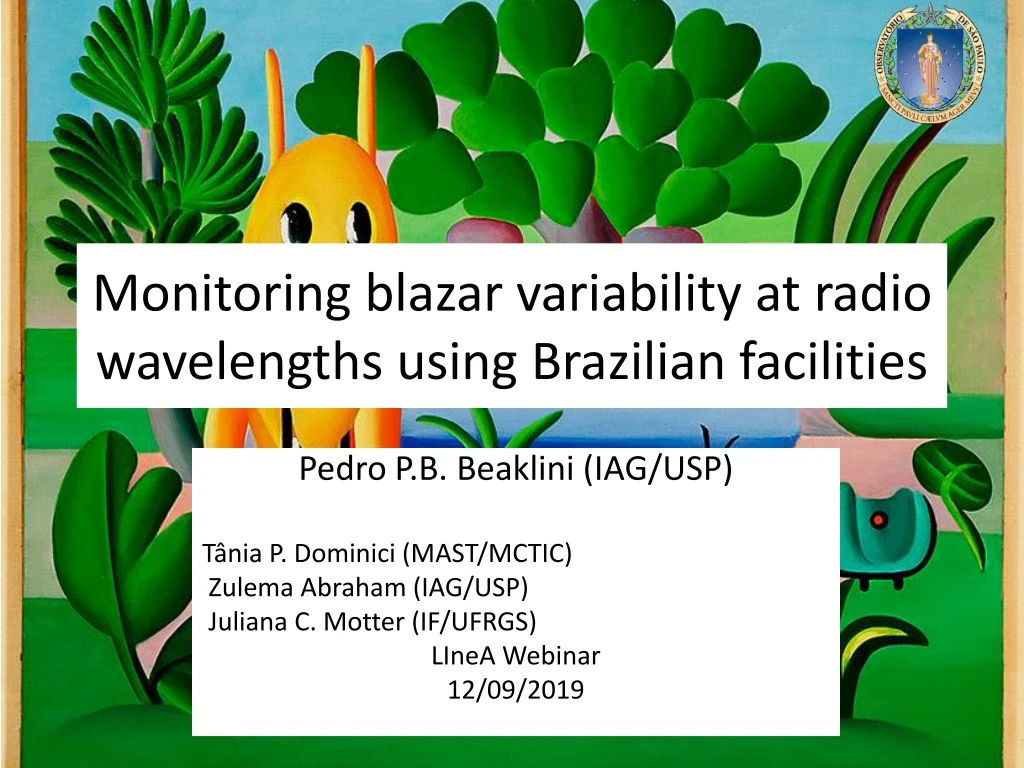
Monitoring blazar variability at radio wavelengths using Brazilian facilities Pedro P.B. Beaklini(IAG/USP) TâniaP. Dominici (MAST/MCTIC) Zulema Abraham (IAG/USP) Juliana C. Motter (IF/UFRGS) LIneA Webinar 12/09/2019
Blazars • High luminosity AGNs • Bright at radio wavelengths. • VVO and BL Lacs -shows variability at all wavelengths. • Small angle between the jet and the line of sight • Therefore, blazars were intensively monitoring at cm wavelength.
Looking “inside” thejet ImageCredit: NRAO website. Gallery https://public.nrao.edu/gallery/agns-seen-at-different-angles/
RelativitiscEffects • Beamingeffects • (Rees 1966; Blandford & Königl 1979) • High - Variability Doppler Factor Lorentz Factor
Superluminal Velocities Components Imageat 22 GHz (VLBA) Source: 3C279 Jet componentevolution Time (Years) Original: Wehrleet al. 2001 (NRAO Gallery) Adapted: Motter 2017 Light-year
Variability (3C273) Soldiet al. 2012
Understanding the Variability • Quiet and Active phase • At last during flare activity • Delays between radio variability and high energy variability • First seen in 3C273, on an IR flare (Robson et al. 1983, Cleeg et al. 1983, Botti & Abraham 1988), Stevens et al. 1994, 1998)
Shock-in-jetmodel Marscher & Gear 1985 Generalizations (e.g.): Hughes, Aller&Aller 1985; Türler, Corvoisier & Paltani 2000;Spadaet al. 2001; Marscher & Jorstad 2010; Hughes, Aller & Aller 2011),
What is goingon? • The shock model • Initially Optically thick component expand and become brighter until turn to a optically thin to a given frequency. • Predict time delays of few days between high energy (gamma and X-Ray) and optical, and few months between high energy and radio Higher time delay for the lower frequencies Radio Frequencies High Energy Delay
Shock-in-jet schema Chidiac et al. 2016
To keep aware • On the source frame, time is different than the obs frame • The duration of each flare is different through the spectrum. Gamma-ray flares are shorter than radio flares • More than simultaneous observations, we need simultaneous monitoring
XXI Century newamountofvariability data • Gamma-Ray Fermi • X-Ray – XMM, Chandra • Optical, IR – SMARTS monitoring (Bonning et al. 2008) • Radio cm – Historic Light Curve • Submillimetric - Few monitoring data from phase calibrators sources. ROPK LLAMA
Blazars SED Before Fermi Rádio Raios-g Fossatiet al. 1998. SED (SpectralEnergyDistribution) dof122 blazares. Before Fermi
Let’s do it • Radio monitoring • Polarimetric monitoring • To compare • Fermi Light curve • Others programs • FAST Comunication
Radio Observations • 7mm (43 GHz) observations at Itapetinga radio observatory (Atibaia, Brazil) • Monthly Basis: • 1510-089: between 2011 and 2013 • 3C279: between 2009 e 2013 • Beam size: 2.4 arc minute (Point source) • Flux Calibrators: VirgoA(Primary) e SgrB2 Main (Secundary)
Scan Method (on-the-fly) • Scan at elevation andazimuthScan time: 20 seconds • Scan Amplitude: 30 arcminuteScanPoints: 81 90 minutes of observation of 3C279
Optical Polarimetric Observation (R Band) • Observations at Pico dos Dias Observatory • Between 2009 and2013 for both sources . • Imaging Polarimeter IAGPOL (Magalhaes et al.1996). • The polarimeter consists of a rotable, achromatic half-wave retarder, followed by a calcite Savart plate. • Data Reduction: IRAF PCCDPACK package (Pereyra 2000).
Can we recovery Magnitude information? 3C279 1510-089 Small and Moderate Aperture Research Telescope System Beaklini 2012 SMARTS data: Bonninget al. 2008
3C273 - March 2010 Setember 2009 180 days delays. High energy coming first Beaklini & Abraham 2014
DCF Method Edelson & Krolik 1988 Beaklini & Abraham 2014
3C273 jet Período de 16 anos Marscehr & Gear 1985 Jortstad et al. 2013 Abraham & Romero 1999
3C273 Beaklini & Abraham 2014
3C279 SMARTS Fermi/LAT Beaklini et al. 2019
3C279 Beaklini et al. 2019
Time Delay Radio-Gamma: 3C279 DCF 150 daysdelay Beaklini et al. 2019
QxU Plane Beaklini et al. 2019
PKS 1510-089 SMARTS Fermi/LAT Beaklini et al. 2017
PKS1510-089 Beaklini et al. 2017
Time Delay – Radio-Gamma:1510-089 Delay of 55 days
PKS1510-089 Beaklini et al. 2017
PD x Magnitude relation Similar result was found by Sasada et al.(2011) and Ikijiri et al.(2011).
ROI Before our monitoring • Most of the time: Only continuum receivers • 43 GHz and 22 GHz • Not easy switch between the frequencies • Pointing and tracking problems
Radio Pointing RádioObservatório do Itapetinga (Pierre Kaufmann) Figure: Meeks et al. 1968
Other issues • 8 years of observation • Calibration • Problems diagnostic • (Receiver, voltmeter, attenuators, GPS, tracking, motor, water)
ROI to ROPK • Partnership Mackenzie-INPE • IAG/USP – instruments • 22 and 43 GHz receivers • Line and continuum • Both bands simultaneous • New Motors
LLAMA • Brasil & Argentina • 12m • Cassegrian Focus • 4.800 m • Atacama Desert • Receivers • 35-50 GHz (1), 66-116 GHz (2-3), 162-211 GHz (5), 211-275 GHz (6),275-373 GHz (7), 620-720 GHz (9)
LLAMA Commissioning Plan ● Test of alarms and security system ● Antenna movements and software verification ● Optical pointing ● Holography ● Receivers installation ● Radio pointing
Holography • Surface Quality • How can we measure? • Can we improve it? • Illumination and Aperture efficiencies • Receiver offset • Optical Problems (?)
How? • Check the radiation response at each part of the dish: • Measuring amplitude and phase. How? Holography • Holography technique consists to measure radiation pattern coming from different parts to determine large errors on its surface.