Download
1 / 29
290 likes | 299 Views
Observing Strategies at Millimetre Wavelengths. Tony Wong, ATNF Narrabri Synthesis Workshop 13 May 2003. Current 3mm System. 3 antennas (CA02, CA03, CA04) with dual polarisation receivers. 2 freq bands: 84.9-87.3 and 88.5-91.3 GHz .

E N D
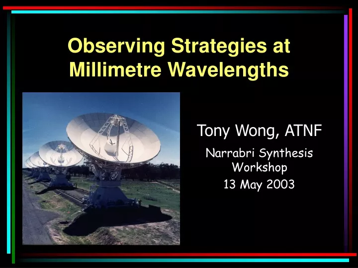
Observing Strategies at Millimetre Wavelengths Tony Wong, ATNF Narrabri Synthesis Workshop 13 May 2003
Current 3mm System • 3 antennas (CA02, CA03, CA04) with dual polarisation receivers. • 2 freq bands: 84.9-87.3 and 88.5-91.3GHz. • Up to 128 MHz bandwidth in each of 2 frequencies (both must be in same band).
Current 12mm System • 6 antennas with dual polarisation receivers. • 2 freq bands: 16.1-18.8 and 20.1-22.4GHz. • If observing 2 frequencies, both must be in same band.
Pending 12mm System • 6 antennas with dual polarisation receivers. • 2 overlapping frequency bands: 16.0-22.4 and 20.0-26.0GHz (ammonia!). • For dual-frequency operation, both freqs must be in same band, and separated by <2.7 GHz (lower band) or <2.3 GHz (upper band). • Available from end of May!
Millimetre interferometry Millimetre interferometry poses special challenges: • Significant atmospheric opacity, much of which is due to H2O vapor (and is hence variable). • Fluctuations in H2O vapor content above the antennas produce atmospheric phase noise that increases with baseline length & with frequency. • Instrumental requirements (e.g. surface, pointing, baseline accuracy) become more severe. • Need more bandwidth to cover same velocity range: 1 MHz lmm km s-1
When to Observe The mm observing season is April to October. Observations outside this period are unlikely to succeed. R. Sault
Atmospheric Opacity TsysTrec + Tsky = Trec + Tatm(1-e-t) Tsys,eff = Tsys et = Trecet + Tatm(et-1) TrmsTsys,eff (nbasBt)–0.5 The variable component of atmospheric opacity t (due to precipitable H2O vapor) is minimised in cold, clear conditions. To try to make optimum use of the array, each mm project is typically assigned a cm“swap” partner. The “swap” is made if the weather during the mm slot is poor.
Phase Stability • Effect of phase noise on a visibility measurement can be expressed as <V>/V0 = exp (– rms2 / 2) where rmsis the RMS phase variation during the averaging time, and V0 is the true amplitude. • For rms=30º (280 mm), <V>/V0=0.87 and the visibility amplitude will be reduced by 13% due to phase noise (also called decorrelation). • rms is a function of weather, frequency, and baseline length: rms Kb0.8
Clear Night, 8pm local time b: 75m 120m 45m 34º 19º rms: 22º
4 hours later (midnight) b: 75m 120m 45m 34º 19º rms: 22º 24º 13º rms: 16º
Advice on Day vs. Night • There is a very strong diurnal effect: phase stability is much better at night, with a few hours’ latency (2 hr after sunrise is much better than 2 hr after sunset). • If phase stability is important (i.e. extended arrays) then may bebetter to observe in morning or evening during “shoulder” season (Apr-May, Sep-Oct)than during afternoon in “peak” season. • Better statistics will be available once a phase monitor is in operation.
Array Configurations • E-W configurations not always ideal for mm obs, which must be done at low airmass (elev > 30°). EW214 d=-35º, beam=7.7” x 2.7”
Array Configurations • N-S or hybrid arrays may improve u-v coverage. H75 beam=6.6” x 4.9”
Array Configurations • Example of combining E-W and N-S arrays. EW367 + 750A + H168 beam=3.3” x 2.8”
Advice on Configurations • Simulate your PSF before writing your proposal. Be sure to include shadowing! • If the emission is likely to be extended, be sure to include short baselines. • Shorter baselines also easier to calibrate.
Gain calibration • Involves observing a bright point source at a known position (e.g., maser or quasar). • Important for tracking phase drifts due to instrumental and large-scale atmospheric effects. • For a quasar, use the maximum possible bandwidth (128 MHz at ATCA). TrmsTsys,eff (nbasBt)–0.5 • Rather than using different correlator config for source vs. cal, employ dual frequency mode (wide & narrow).
Gain calibration • For a maser, use a bandwidth that gives you adequate freq resolution to resolve the line.
Choosing your calibrator A good calibrator is within 15º of your target source and has a flux in the ATCA catalogue of >1 Jy.
Choosing your calibrator The reasons for these guidelines are: • Catalogued mm fluxes unreliable, and sources <1 Jy are often <<1 Jy. • If the calibrator is more than 15º away, you may be observing it through a very different H2O column, and will be more susceptible to antenna position (baseline) errors. Holdaway (1992 ALMA memo) estimates that the mean distance between a source and calibrator at 115 GHz will be 7º x S0.75, where S is the flux cutoff in Jy.
How often and how long? Don’t want to spend too much time calibrating! Need to find compromise between: • Errors in gain solution due to S/N on cal • Errors due to atmospheric changes • Time lost due to calibrator observations Usually calibrating every 20-30 minutes is adequate for baselines < 100m. For a 1 Jy source, to achieve a S/N of 10 in each baseline and polarisation requires just 1 minute’sintegration in good weather.
Desai 1998 How often and how long? Ideally, we’d like to calibrate faster than troposphere moves across the array. But with typical wind speeds of ~10 m/s, this would require calibrating every 20s for a 100m baseline!
Desai 1998 How often and how long? Less frequent calibration still useful: removes fluctuations with size scales > beff ~ vatcyc/2 ~ 300m x (tcyc/min). Rule of thumb: for baselines twice as long, calibrate the phase twice as often.
Observing a test calibrator In poor weather or when usinglong baselines, it may be unclear whether a non-detection is due to source weakness or to atmospheric phase decorrelation. Procedure:observe a weaker (but detectable) “test” quasar near your source, in addition to a stronger quasar as the phase calibrator. If phase gains applied to the test quasar yield a good detection, your phase calibration is probably adequate.
Other required calibrations Paddle (vane) calibration: measures Tsys,eff. Changes quickly during rise & set or in cloudy weather (repeat every ~15 min), more slowly near transit (~30 min).
Other required calibrations Pointing calibration: refines antenna pointing by doing a “cross” pattern around a bright source. At least once an hour or when moving to a different part of sky. • Primary beam FWHM is only 36” at 86 GHz! • A 10º shift in elevation can produce a ~5” shift in pointing: must choose a nearby source!
Other required calibrations Bandpass calibration: determines amplitude and phase on a strong point source as a function of frequency (once during project).
Other required calibrations Flux calibration: observe thermal continuum emission from an unresolved planetonce during project, to set absolute flux scale. MIRIAD task plplt
Hexagonal grid Rectangular grid Multi-field imaging Due to the small size of the ATCA beam at mm wavelengths, it will often be desirable to combine several fields (mosaic). But, pointing errors and uncertainties in the beam shape make this difficult at present.
Parting Thoughts • Best to observe sources that you believe will be detectable in 4 hours or less integration time. • Time flies when you’re stuffing around – don’t modify your observing strategy midway unless there’s an obvious mistake. • Use loops when possible: have a sequence of pointing, calibration, and on-source scans that can be repeated many times. • Keep an eye on slew times and shadowing (even by idle antennas!). Don’t observe at elevations >85º. • Especially at 3mm, record Tsys and pointing offsets in log – useful to diagnose problems in reduction.