Download
1 / 66
700 likes | 819 Views
PHY1012F Kinematics. Gregor Leigh gregor.leigh@uct.ac.za. KINEMATICS. Learning outcomes: At the end of this chapter you should be able to…. Interpret, draw and convert between position, velocity and acceleration graphs for 1-d motion.

E N D
PHY1012FKinematics Gregor Leighgregor.leigh@uct.ac.za
KINEMATICS Learning outcomes:At the end of this chapter you should be able to… • Interpret, draw and convert between position, velocity and acceleration graphs for 1-d motion. • Use an explicit problem-solving strategy for kinematics problems. • Apply appropriate mathematical representations (equations) in order to solve numerical kinematics problems involving motion in one dimension.
MOTION IN ONE DIMENSION We shall standardise on the following sign conventions: • The positive end of the x-axis points to the right; The positive end of the y-axis points upwards. • y • x
MOTION IN ONE DIMENSION We shall standardise on the following sign conventions: • Positions left of the y-axis have negative x values; Positions right of the y-axis have positive x values. • Positions below the x-axis have negative y values;Positions above the x-axis have positive y values. x>0; y>0 • y x<0; y>0 x=0; y>0 0 • x x<0; y=0 x>0; y<0 x<0; y<0
MOTION IN ONE DIMENSION We shall standardise on the following sign conventions for representing directions: • Vectors pointing to the right (or up) are positive; Vectors pointing to the left (or down) are negative. • y • x • NB: The signs represent the directions. The magnitudes of vectors can never be negative!
MOTION IN ONE DIMENSION In 1-d the relationship between acceleration and velocity simplifies to… • When is zero, velocity remains constant. • If and have the same sign, the object is speeding up. • If and have opposite signs, the object is slowing down.
The slope at a point on a position-vs-time graph of an object is Athe object’s speed at that point Bthe object’s acceleration at that point Cthe object’s average velocity at that point Dthe object’s instantaneous velocity at that point Ethe distance travelled by the object to that point
POSITION GRAPHS Plotting a body’s position on a vertical axis against time on the horizontal axis produces a position-vs-time graph, or position graph… 1 frame per minute • x (m) 0 100 200 300 400 • x (m) 400 200 0 0 2 4 6 • t (min)
POSITION GRAPHS Plotting a body’s position on a vertical axis against time on the horizontal axis produces a position-vs-time graph, or position graph… • x (m) 0 100 200 300 400 1 frame per minute • x (m) 400 200 0 0 2 4 6 • t (min)
INTERPRETING POSITION GRAPHS It is essential to remember that motion graphs are abstract representations of motion – they are NOT pictures! At 40 min the car starts moving back to the right. The car reaches the origin once more at 80 min. After 30 min the car stops for 10 min at a position 20 km to the left of the origin. During the first 30 min the value of x changes from +10 km to 20 km, indicating that the car is moving to the left. At t = 0 the car is 10 km to the right of the origin. The following graph represents the motion of a car along a straight road… Describe the motion of the car. • x (km) 10 • t (min) 0 20 40 60 80 –10 –20
UNIFORM MOTION Straight-line motion in which equal displacements occur during any successive equal-time intervals is called uniform motion. s (m) 6 s = 4 m 4 2 0 t (s) 0 2 4 6 t = 6 s Motion diagram: Position graph:
UNIFORM MOTION Straight-line motion in which equal displacements occur during any successive equal-time intervals is called uniform motion. s (m) t = 4 s Motion diagram: 6 4 Position graph: s = 6 m 2 0 t (s) 0 2 4 6 An object’s straight line motion is uniform if and only if its velocity vx (or vy) is constant and unchanging.
POSITION GRAPHS OF UNIFORM MOTION x (m) B t (s) x (m) Body A is travelling to the right at constant speed… A t (s) Body B is… travelling to the left/right and is going slower/faster than A. (Assume same axes scales.)
POSITION GRAPHS OF UNIFORM MOTION Summary: Zero slope zero velocity. (Object is stationary.) Steeper slopes faster speeds. Negative slope negative velocity (ie vx is left/vy is down). The sign (negative or positive) refers only to the direction of the velocity, and has nothing to do with its magnitude.
POSITION GRAPHS OF UNIFORM MOTION Summary: Zero slope zero velocity. (Object is stationary.) Steeper slopes faster speeds. Negative slope negative velocity (ie vx is left/vy is down). The sign (negative or positive) refers only to the direction of the velocity, and has nothing to do with its magnitude. The slope is a ratio of intervals, x/t, not coordinates, x/t. Remember: Position graphs are abstract representations! We are concerned with the physically meaningful slope [in m/s], not the actual slope of the graph on paper. PHY1012F 15
Describe carefully (and quantitatively) the motion of the basketball player depicted by this position graph. 0 1 2 3 4 x (m) 6 4 2 0 t (s)
THE MATHEMATICS OF UNIFORM MOTION The velocity of a uniformly moving object tells us the amount by which its position changes during each second. s (m) sf s si t (For uniform motion) t (s) ti tf
MULTI-REPRESENTATIONAL PROBLEM-SOLVING Bob leaves home in Chicago at 09:00 and travels east at a steady 100 km/h. Susan, 680 km to the east in Pittsburgh, leaves at the same time and travels west at a steady 70 km/h. Where will they meet? Pictorial representation: • (ax)B = 0 • (ax)S = 0 Bob Bob • x • 0 • (x1)B, (vx)B, t1(x1)S, (vx)S, t1 • (x0)S, (vx)S, t0 • (x0)B, (vx)B, t0 (x0)B = 0 km (vx)B = +100 km/h t0 = 0 h t1 is when (x1)B = (x1)S (x0)S = +680 km (vx)S = –70 km/h (x1)B = ?
MULTI-REPRESENTATIONAL PROBLEM-SOLVING Bob leaves home in Chicago at 09:00 and travels east at a steady 100 km/h. Susan, 680 km to the east in Pittsburgh, leaves at the same time and travels west at a steady 70 km/h. Where will they meet? Physical representation: Chicago meet Pittsburgh
Bob leaves home in Chicago at 09:00 and travels east at a steady 100 km/h. Susan, 680 km to the east in Pittsburgh, leaves at the same time and travels west at a steady 70 km/h. Where will they meet? MULTI-REPRESENTATIONAL PROBLEM-SOLVING Graphical representation: • x (km) Susan 600 400 200 Bob 0 • t (h) tmeet 0
Bob leaves home in Chicago at 09:00 and travels east at a steady 100 km/h. Susan, 680 km to the east in Pittsburgh, leaves at the same time and travels west at a steady 70 km/h. Where will they meet? MULTI-REPRESENTATIONAL PROBLEM-SOLVING sf = si + vst Mathematical representation: • (x1)B = (x0)B + (vx)B(t1– t0) • (x1)S = (x0)S + (vx)S(t1– t0) • They meet when (x1)B = (x1)S = (vx)Bt1 = (x0)S + (vx)St1 i.e. (vx)Bt1 = (x0)S + (vx)St1 • (x1)B = (vx)Bt1 = 100 km/h 4.0 h = 400 km east of Chicago
INSTANTANEOUS VELOCITY Adjusting the time interval between “movie frames” of the horizontally orbiting tennis ball alters the average velocity vectors and the information they convey…
INSTANTANEOUS VELOCITY Adjusting the time interval between “movie frames” of the horizontally orbiting tennis ball alters the average velocity vectors and the information they convey… The longer the time interval, the less “real” the representation: (Especially if the “background” information is removed.)
INSTANTANEOUS VELOCITY Conversely, the shorter the time interval, the more the vectors tend to show us what the ball is really doing – rather than merely depicting “average” behaviour for that time interval. As t gets smaller and smaller, approaches a limit – a constant value representing the instantaneous velocity at that point in time. Mathematically:
DERIVATIVES The limit, , is called the derivative of s with respect to t. The derivative of a sum is the sum of the derivatives: In general (using an arbitrary function as a template), if u = ctn, to find the derivative of u (with respect to t)… • Multiply the expression by the existing index. • Subtract 1 from the index. ctn n –1 E.g. i.e.
INSTANTANEOUS VELOCITY The same process of shrinking the time interval to determine the instantaneous velocity at one particular time can also be applied to linear motion. In this case, however, it is more helpful to make use of a position graph rather than a motion diagram…
The motion diagram represents an object whose speed is NOT constant, but increases uniformly each second: INSTANTANEOUS VELOCITY • s (m) 16 12 8 4 • t (s) 0 0 2 4 6 8 1 frame per second • s (m) 0 2 4 6 8 10 12 14 16 (Plotting uniformly accelerated motion against time results in a parabolically-shaped position graph.)
INSTANTANEOUS VELOCITY The ratio gives the average velocity, , for that particular time interval, represented graphically by the slope of the dotted line. • s (m) The larger t, the less detailed the information… • s • s • s • t • t • t • t (s)
INSTANTANEOUS VELOCITY Conversely, if we let the time interval either side of time t shrink towards the limit (t0), we get the instantaneous velocity at time t. • s (m) On a position graph this corresponds to the slope of the tangent to the curve at time t. Mathematically: • t (s) • t
INSTANTANEOUS vs AVERAGE VELOCITY Note that (for uniform acceleration) the average velocity for a whole time interval is the same as the instantaneous velocity at time t in the middle of the interval… …as illustrated by the parallel slopes of the dotted lines on the position graph. • s (m) • t (s) • t
POSITION GRAPHS VELOCITY GRAPHS • x (m) 10 • t (s) 0 2 4 6 8 –10 –20 • vx(m/s) 5 0 • t (s) 2 4 6 8 –10 Velocity is equivalent to the slope of a position graph. E.g. A car travels along a straight road… For the first 3 s the is x slope velocity t
POSITION GRAPHS VELOCITY GRAPHS Velocity is equivalent to the slope of a position graph. • x (m) E.g. A car travels along a straight road… 10 • t (s) 0 Between 3 s and 4 s the is 2 4 6 8 slope velocity –10 –20 • vx(m/s) 5 0 • t (s) 2 4 6 8 –10
POSITION GRAPHS VELOCITY GRAPHS Velocity is equivalent to the slope of a position graph. • x (m) E.g. A car travels along a straight road… 10 • t (s) 0 Between 4 s and 8 s the is 2 4 6 8 slope velocity –10 x –20 t • vx(m/s) 5 0 • t (s) 2 4 6 8 –10
POSITION GRAPHS VELOCITY GRAPHS • x (m) 10 • t (s) 0 2 4 6 8 –10 –20 • vx(m/s) 8 4 0 • t (s) 2 4 6 8 Velocity is equivalent to the slope of a position graph. E.g. A car travels along a straight road… For the first 3 s theincreases steadily from zero to 7 m/s. slope velocity
POSITION GRAPHS VELOCITY GRAPHS • x (m) 10 • t (s) 0 2 4 6 8 –10 –20 • vx(m/s) 8 4 0 • t (s) 2 4 6 8 Velocity is equivalent to the slope of a position graph. E.g. A car travels along a straight road… From 3 s to 6 s theremains a steady 7 m/s. slope velocity
POSITION GRAPHS VELOCITY GRAPHS • x (m) 10 • t (s) 0 2 4 6 8 –10 –20 • vx(m/s) 8 4 0 • t (s) 2 4 6 8 Velocity is equivalent to the slope of a position graph. E.g. A car travels along a straight road… Between 6 s and 7 s thequickly decreases to 0… slope velocity …and remains there.
THREE-MINUTE PAPER On a smallish piece of paper (which you’re going to fold in half), answer the following questions: What have you learnt so far? What still confuses you the most? Are you having fun? (If not, why not?!)
FINDING POSITION FROM VELOCITY In the previous chapter we showed that a body’s position can be determined from its velocity using . • vs(m/s) 8 4 0 • t (s) 2 4 6 8 Graphically, the change in position (s =vt) is given by the area “under” a velocity graph: During the time interval 2 s to 8 s the body travels a distance v t
FINDING POSITION FROM VELOCITY In the previous chapter we showed that a body’s position can be determined from its velocity using . • vs(m/s) 8 4 0 • t (s) 2 4 6 8 PHY1012F Graphically, the change in position (s =vt) is given by the area “under” a velocity graph: Even if the velocity varied (uniformly) during the time interval, s could still be determined by summing the “bits”: s1 s3 s2 39
FINDING POSITION FROM VELOCITY If the velocity varies non-uniformly during the interval… …we can approximate the motion with a series of constant velocity intervals. The total area under the graph is approximately • vs(m/s) (vs)1 (vs)2 s1 s2 t t • t (s) ti tf
FINDING POSITION FROM VELOCITY Once again we apply calculus, shrinking the t’s to obtain more and more accurate approximations… • vs(m/s) until, as t 0, s1 s2 s4 s3 • t (s) So ti tf
INTEGRALS is called the integral of vs dt from ti to tf. Since it has two definite boundaries (ti and tf), it is known as a definite integral. In general (using an arbitrary function as a template), The integral of a sum is the sum of the integrals:
DIFFERENTIATION AND INTEGRATION FOR DUMMIES n +1 To differentiate u = ctn … • Multiply the expression by the existing index. • Subtract 1 from the index. ctn n –1 To integrate u = ctn … • Add 1 to the index. • Divide the expression by the new index. • Evaluate the integral at the upper limit, and... • subtract the lower limit value of the integral. ctn +1
FINDING POSITION FROM VELOCITY A body which starts at position xi= 30 m at time ti, moves according to vx= (–5t + 10)m/s. • vx(m/s) 10 0 –10 • t (s) 2 4 6 –20 • Where does the body turn around? • At what time does the body reach the origin?
FINDING POSITION FROM VELOCITY A body which starts at position xi= 30 m at time ti, moves according to vx= (–5t + 10)m/s. • Where does the body turn around? • At what time does the body reach the origin? • and • Substitute t = 2 and solve for x. • Substitute x = 0 and solve for t.
VELOCITY GRAPHS ACCELERATION GRAPHS • vx(m/s) 6 0 0 • t (s) • t (s) 3 3 6 6 9 9 12 12 –6 • ax(m/s2) 1 –1 –2 Acceleration is equivalent to the slope of a velocity graph. E.g. A car travels along a straight road… For the first 6 s the is slope acceleration
VELOCITY GRAPHS ACCELERATION GRAPHS • vx(m/s) 6 0 0 • t (s) • t (s) 3 3 6 6 9 9 12 12 –6 • ax(m/s2) 1 –1 –2 Acceleration is equivalent to the slope of a velocity graph. E.g. A car travels along a straight road… For the last 6 s the is slope acceleration acceleration
SUMMARY OF GRAPHS OF MOTION Constant +ve velocity • s • s • s • t • t • t • vs • vs • vs • vis • vfs • vis • vis • vfs • t • t • t • as • as • as • 0 • t • 0 • 0 • t • t Increasing +ve velocity Decreasing +ve velocity
SUMMARY OF GRAPHS OF MOTION Constant –ve velocity • s • s • s • t • t • t • vs • vs • t • t • vfs • vis • vfs • vis • as • as • vs • as • 0 • 0 • t • t • 0 • 0 • t • t Increasing –ve velocity Decreasing –ve velocity
KINEMATIC EQUATIONS OF CONSTANT a By definition, vs(m/s) vfs vs = ast ½as(t)2 vis Hence: vfs = vis + ast vis vist t (s) ti tf t sf = si + area under v-graphbetween tiand tf . Hence: sf = si + vist + ½as(t)2 And, substituting t = (vfs– vis)/as: vfs2= vis2 + 2ass