1 / 0

External Costs of Air Pollution

Ari Rabl , ARMINES/Ecole des Mines de Paris ari.rabl@gmail.com and www.arirabl.org October 2014 External Costs = cost that are not taken into account by the market e.g. damage costs of pollution, if polluter does not pay, = costs imposed on others

roxy
Download Presentation

External Costs of Air Pollution

An Image/Link below is provided (as is) to download presentation Download Policy: Content on the Website is provided to you AS IS for your information and personal use and may not be sold / licensed / shared on other websites without getting consent from its author. Content is provided to you AS IS for your information and personal use only. Download presentation by click this link. While downloading, if for some reason you are not able to download a presentation, the publisher may have deleted the file from their server. During download, if you can't get a presentation, the file might be deleted by the publisher.

E N D

Presentation Transcript


  1. Ari Rabl, ARMINES/Ecole des Mines de Paris ari.rabl@gmail.com and www.arirabl.org October 2014 External Costs = cost that are not taken into account by the market e.g. damage costs of pollution, if polluter does not pay, = costs imposed on others perspective of society  perspective of individual Need government regulations to internalize external costs (make polluter take into account the external cost, i.e. act as if polluter and victims were the same) Part of the damage costs are already internalized by current regulations, and some economists define external cost as only that part of the damage cost that still remains to be internalized (but that is difficult to determine and very uncertain). In practice most people now refer to the entire damage cost of pollution as “external cost”.

    External Costs of Air Pollution

  2. Most air pollution, (and a large part of all pollution) is directly or indirectly linked to energy (electricity, heat, transport) Combustion of fossil fuels: CO2 ( global warming) NOx( acid rain, tropospheric O3, health impacts) SOx( acid rain, health impacts) black smoke, particles ( health impacts) other: nuclear waste CFCs (insulation, refrigeration) ( stratospheric O3 hole) land use (power plants, mines, wastes, ...) accidents (mines, Chernobyl, ...) Noise etc …

    Sources of Pollution

  3. Difficult choices(high costs): e.g. pay extra for clean energy? photovoltaics? "zero emission" vehicles? fuel cell car? improved flue gas treatment? e.g. catalytic reduction of NOx close a factory with high pollution? cancers or jobs? Excessive spending for environmental protection takes money away from other worthy causes, such as education and public health Cost-benefit analysis (CBA) can help optimize allocation of scarce resources, i.e. compare costs and benefits of pollution abatement

    How much is clean air worth?

    pollution abatement = measures to reduce pollution
  4. = Ranking of abatement measures in terms of their result/cost ratio. Example: CO2 abatement in EU by 2020 (reference: IIASA, GAINS model) Each segment of the curve represents marginal cost (€/tCO2) and contribution to abatement (GtCO2/yr) of a particular abatement measure, e.g. replacement of incandescent lighting by fluorescent.

    Cost-Effectiveness Analysis (CEA)

    CEA does not tell us how far we should abate; for that we need to know also the benefits (cost-benefit analysis)
  5. 1) Zero pollution: Unrealistic, our economy could not function 2) Stay below threshold of harmful impacts: OK if there is such a threshold (often the case for ecosystem impacts) but for many pollutants/impacts there is no such threshold, e.g. greenhouse gases, health impacts of NOx, PM, SO2, O3, carcinogens, … 3) Precautionary principle: no useful guidance 4) Minimize the total social costCtot(E) = Cdamage(E) + Cabatement(E) as function of pollution emission E  Marginal damage cost = - marginal abatement cost

    Criteria for DeterminingOptimal Level of Pollution

  6. only a general guideline (“Think before you act!”), no advice for specific problems Must be used with a great deal of precaution, to avoid unexpected consequences e.g. Overestimating risks of nuclear implies increased global warming and conventional pollution Overestimation of mortality costs of pollution implies increased mortality through indirect impacts (“poverty kills”) Whose risks, whose precaution?  We need expectation value of damage costs, except for cases where valuation is very non-linear function of damage (e.g. very large accident, or irreversible damage)

    The Precautionary Principle

  7. Example: costs of CO2 General case (almost always): Marginal abatement costdecreases with E Typical case for classical air pollutants: Marginal damage cost = constant for CO2: Marginal damage cost increases with E

    Optimal level of pollution, cont’d

    At optimum
  8. Information Needs of Policy Makers Environmental policies need to target specific pollution sources General policies, e.g. ambient air quality standards, are not sufficient Policy makers must tell each polluter how much to reduce the emission of each pollutant (e.g, NOx from cars = precursor of O3 and PM10)  Theyneed to know impact (cost) of emitted pollutant For some decisions the also need LCA results, e.g. choice between nuclear and coal, electric or fuel cell vehicles (“pollution elsewhere vehicles”), hydrogen economy
  9. ExternE = “External Costs of Energy” Series of research projects funded by European Commission DG Research, since 1991 (until 1995 with ORNL/RFF) >200 scientists in all countries of EU (A. Rabl is one of the key participants) Major publications 1995, 1998, 2000, 2004, and 2008 (definitive results) www.externe.info Methodology 1) Life Cycle Assessment of process or product chain (LCA) 2) Site specific Impact Pathway Analysis (IPA)

    Towards an answer: the ExternE Project Series of the EC

  10. to calculate damage of a pollutant emitted by a source Impacts are summed over entire region that is affected (Europe) and all damage types that can be quantified: health loss of agricultural production damage to buildings and materials Result: €/kg of pollutant Multiply by kg/kWh to get €/kWh

    Impact Pathway Analysis

  11. For many persistent pollutants (dioxins, As, Cd, Cr, Hg, Ni, Pb, etc) ingestion dose is about two orders of magnitude higher than inhalation

    Pathways for Dioxins and Toxic Metals

  12. Relation between impact pathway analysis and current practice of most LCA, illustrated for the example of electricity production.

    Life cycle analysis (LCA)

    LCA should include site-specific IPA with realistic exposure-response functions and monetary valuation - but that’s usually not done in current practice.
  13. Comparison LCIA  ExternE Impact 2002+ is the most complete LCIA (life cycle impact assessment) Impact 2002+, like most LCA: no monetary valuation, and tries to include everything (even if the ERFs are dubious) whereas ExternE focuses on items with the largest damage cost, trying to be as realistic as possible
  14. Comparison LCIA  ExternE
  15. Comparison LCIA  ExternE
  16. Very limited and simplified list

    Comparison of tools for evaluating environmental policy options

  17. For non-market goods: based on Willingness-to-pay (WTP) to avoid a loss e.g. VSL = “Value of Statistical Life” (a better name VPF = value of prevented fatality) = WTP to avoid risk of an anonymous premature death typical values used in EU and USA 2-5 M€ Value of a Life Year (VOLY) due to air pollution = 40,000 €

    Monetary valuation

    Methods for valuation of non-market goods: Contingent valuation (survey of individuals) analysis of consumer choices (e.g. lower rent for noisy apartments, travel cost, higher wage for higher risk, etc)
  18. Land use: Serious impact on ecosystems and biodiversity (biodiversity decreases if size of an ecosystem is reduced, e.g. if it is cut by a road) Very site-specific. Storage of waste (nuclear and conventional): Difficulty: damage depends on future management of storage, with new technologies leakage during the operation of the facility is negligible, but what will happen in the future? need scenarios ExternE: assessment of waste storage for nuclear, but so far not for fossil fuel chains

    Land use, waste storage

  19. ExternE 1995 and 1998: Very low damage costs (lowest of all except wind, solar and for some sites hydro) but … Risks of nuclear proliferation and terrorism: Temptation to increase profit and economies of scale by selling the technology to countries that lack sufficient safeguards (the link nuclear power -> military is undeniable) Risks of major nuclear accident: ExternE 1995: Extremely small with new technologies, but public perception? Long term storage of waste: No problem as long as storage site is supervised. But is our society stable enough in the long term? Risks imposed on future generations: nuclear waste vs. CO2

    Nuclear power

  20. Health impacts of pollution

    Are the observed impacts due to particles or due to NO2 or SO2?
  21. Health impacts of pollution, cont’d
  22. Health effects of air pollution Healthy individuals have sufficient reserve capacity not to notice effects of pollution, but the effects become observable at times of low reserve (during extreme physical stress, severe illness, or last period of life) Pollution reduces reserve capacity  Mortality impact is not the loss of a few months of misery at the end but the shrinking of the entire quality of life curve (“accelerated aging”) In large population there are always some individuals with very low reserve capacity  impacts observable
  23. Epidemiology: comparing populations with different exposures. 2) Laboratory experiments with humans: exposure in test chambers with controlled concentration of air pollutants (but this approach is very limited because of ethical constraints). 3) Toxicology: a) Expose animals (usually rats or mice) to a pollutant; sample sizes are usually very small compared to epidemiological studies, and the animals are selected to be as homogenous as possible (unlike real populations). Extrapolation to humans??? b) Expose tissue cultures to pollutants. Extrapolation to real organism???

    Approaches to measure health impacts

  24. Epidemiology: can measure impacts on real human populations, by observing correlations (“associations”) between exposure and impact. But in most cases the uncertainties are very large. Is the impact due to the pollutant or due to other variables that have not been taken into account (the problem of “confounders”, especially smoking)? Toxicology: can identify mechanisms of action of the pollutants. For many substance tests with animals are the only way to identify carcinogenic effects. Toxicology can also suggest new questions to be investigated by epidemiology. The two approaches are complementary.

    Approaches to measure health impacts, cont’d

  25. (for air pollutants also known as exposure-response functions or concentration response functions) Crucial for calculating impacts of a pollutant. Note: a) most epidemiological studies do not report explicit DRFs but only a relative risk (= increase in occurrence of a health impact due to increase of exposure). To obtain DRF one also needs data on background rates of occurrence. b) Watch out for consistency of DRF with the specification of exposure (calculated by dispersion models) and with monetary valuation. E.g. is exposure specified as hourly peak or as 24 hr average?

    Dose-response functions (DRFs)

  26. Possible functional forms at low doses Linearity without threshold is the most plausible assumption for NO2, PM, O3, SO2, and carcinogens (including radiation)

    Form of exposure-response functions (ERF) at low doses (also known as dose-response function)

    Difference between ERFsfor individuals and for populations Toxicology: small samples of identical individuals  threshold Epidemiology: real populations with large variations of sensitivity  often no threshold
  27. In terms of costs, the most important emitted pollutants (apart from greenhouse gases) are PM, SO2 (precursor of sulfate aerosols), NOx and VOC (precursors of O3). About 65% of their total damage cost is due to mortality! About 15% due to chronic bronchitis, About 15% due to other health impacts, Only a few % due to agricultural losses, and damage to buildings

    Importance of Mortality

  28. Loss of Life Expectancy due to Air Pollution In EU and USA typical concentrations of PM2.5 around 20 - 30 g/m3 LE loss 8 months Reasonable policy goal during coming decades: reduction by about 50% Life expectancy (LE) gain about 4 months Other countries, e.g. China: concentrations ~2 to 3higher  total LE loss ~2 to 4 years To put this in perspective with other public health risks: Smokers lose about 5 to 8 years on average Rule of thumb: each cigarette reduces LE by about the duration of the smoke Air pollution (in EU and USA) equivalent to about 4 cigarettes/day
  29. Key issue for environmental policy because most of total damage cost of pollution is due to mortality

    How to measure the impacts and costs of air pollution mortality

    Loss of life expectancy  VOLY VOLY = Value of a Life Year or Number of deaths  VPF VPF = Value of Prevented Fatality (=VSL = “Value of Statistical Life”) =“willingness-to-pay to avoid an anonymous premature death” ??? ??? VPF used foraccidents, Loss of LE for public health
  30. VPF based on accidents (large LE loss/death)  air pollution 2) True number of air pollution deaths is not knowable(at current state of science): “air pollution death” = death advanced by air pollution not a primary cause of death Cohort studies cannot distinguish if observed mortality due to everybody losing a little or a few a lot if everybody loses some LE, all deaths are “air pollution deaths” The calculation of number of deaths from cohort studies is wrong because it does not take into account change in age structure during future years Number of deaths from conventional time series studies includes only acute effects (very small LE loss compared to total) 3) LE loss due to air pollution can be determined

    Number of deaths  VPF:mediagenic but wrong

  31. Other Effects of Air Pollutants
  32. Global warming, causes

  33. Global temperature and sea level, past

    From: http://www.ipcc.ch/pdf/assessment-report/ar4/wg1/ar4-wg1-ts.pdf
  34. Scenarios and temperature change

    SRES = Special Report on Emission Scenarios From: http://www.ipcc.ch/pdf/assessment-report/ar4/syr/ar4_syr.pdf
  35. For the A1B scenario and comparing the period 2080 to 2099 with the control period 1980 to 1999

    Predicted changesin precipitation

    From: http://www.ipcc.ch/pdf/assessment-report/ar4/wg1/ar4-wg1-chapter11.pdf
  36. Physical impacts of global warming

    Ref: http://www.ipcc.ch/pub/wg2TARtechsum.pdf (Table.TS-1) Pre-industrial concentration = 280 ppm Changes of heating and cooling Changes of agricultural production Increased incidence of tropical diseases (malaria, dengue fever, …) Migrations of displaced populations Extreme weather events (costs = ??) Ecosystem impacts: species extinction, … (costs = ????) Social and political problems, especially in poor countries (costs = ????) Changes in ocean circulation (could be abrupt, ~years) Some will gain but most will lose
  37. Various estimates for 2xCO2 loss on the order of 1 to 3 % of gross world product Cost per ton of CO2 depends on discount rate and other controversial assumptions especially “value of life” in developing countries (where most of the damage will occur) mainstream estimates are around of 20 €/t of CO2 (but is it agreement by imitation?) Valuations by ExternE ExternE 1998: Calculations by ExternE team: 3.8-139 €/tCO2 18-46 €/tCO2 (“restricted range”, geometric mean 29 €/tCO2 ) ExternE 2000: 2.4 €/tCO2 ExternE2008: 21 €/tCO2

    Monetary valuation of global warming

  38. Studies in 2004 and 2005 (literature review and detailed modeling)

    Global warming cost, recent estimates by UK

    Report by Stern et al in 2006 Damage cost around 85 $/tCO2 (65 €/tCO2)
  39. Current emissions and implications of a CO2 tax

    Germany 10 tCO2/yr France 6 tCO2/yr If tax = 20 €/tCO2: for 6 tCO2/yr per per person cost = 120 €/yr per person (France) Implication for electricity (note current average price ~11 cents/kWh): gas (combined cycle) 0.4 kg/kWh0.8 cents/kWh coal (steam turbine) 0.9 kg/kWh1.8 cents/kWh Stabilization at 550 ppm
  40. Reduce emissions Shift to renewables or nuclear Increase efficiency of fossil energy use carbon sequestration (storing CO2 in depleted reservoirs of natural gas or oil, in aquifers, deep ocean, …) Life style changes, e.g. eat less red meat, more vegetarian food Adaptive measures to reduce impacts, e.g. develop drought resistant crops change crops build dikes

    What do to about global warming?

  41. Impacts 1) Global warming (CO2, CH4, N2O) 2) NOx, SO2, PM etc(primary & secondary pollutants) Health (morbidity: ~ 30%, mortality: ~65% of total cost of these pollutants) The rest is only a few %: Buildings & materials Agricultural crops acidification & eutrophication 3) Other burdens Amenity (noise, visual impact, recreation) supply security Technologies Energy: coal, lignite, oil, gas, biomass, PV, wind, hydro, nuclear Waste: incineration, landfill Transport: cars, trucks, bus, rail, ship, (planes)

    Impacts and Technologies evaluated by ExternE

  42. Local + regional dispersion models Linear dose-response functions for health (no threshold): Mostly PM2.5, PM10, O3 A few for SO2 and NO2 Sulfates are assumed like PM10, Nitrates like 0.5  PM10 also As, Cd, Cr, Hg, Ni and Pb Mortality in terms of LLE (loss of life expectancy) rather than number of deaths Monetary valuation based on Willingness-to-pay (WTP) to avoid a loss: Value of a Life Year (VOLY) due to air pollution = 40,000 € Cancers 2M€/cancer, based on VSL = 1 M€ (VSL = “Value of Statistical Life” = WTP to avoid risk of an anonymous premature death; typical values used in EU and USA 1-5 M€)

    Key Assumptions of ExternE

  43. Damage Cost per kg of Pollutant,and uncertainty (error bars),according to ExternE [2008]

    h = stack height PMco = 2.5 – 10 mm 21 €/tCO2 Note: somewhat different numbers in different publications (due to progress in methodology)
  44. Results for Power Plants Typical numbers for EU27 [ExternE 2008]. Market price ~11cents/kWh (France 2011)
  45. Net impact very dependent on energy recovery. Some examples: Results for Waste Treatment Energy recovery replaces H = heat E = electricity g= gas o = oil c = coal Compare with private costs: Incineration ~ 100€/twaste Landfill ~ 50€/twaste Other = toxic metals (mostly Hg and Pb) and dioxins (very small with current regulations)
  46. There are many different models for atmospheric dispersion and chemistry, with different objectives: e.g. microscale models (street canyons), local models (up to tens of km), regional models (hundreds to thousands of km), short term models for episodes, long term models for long term (annual) averages. For damage costs of air pollution, note that the dose-response functions for health (dominant impact) are linear  only the long term average concentration matters For agricultural crops and buildings they are nonlinear, but can be characterized in terms of seasonal or annual averages only the long term average concentration is needed Dispersion of most air pollutants is significant up to hundreds or thousands of km need local + regional models for long term average concentrations (they tend to be more accurate than models for episodes)

    Atmospheric models for damage costs

  47. Depends on meteorological conditions: wind speed and atmospheric stability class (adiabatic lapse rate, see diagrams at left)

    Dispersion of Air Pollutants

  48. for atmospheric dispersion (in local range < ~50 km)

    Gaussian plume model

  49. concentration c at point (x,y,z) Underlying hypothesis: fluid with random fluctuations around a dominant direction of motion (x-direction)

    Gaussian plume model

    c=concentration, kg/m3 Q=emission rate, kg/s v= wind speed, m/s, in x-direction y=horizontal plume width z=vertical plume width he=effective emission height Source at x=0,y=0 Plume width parameters y and z increase with x
  50. There are several models for estimating y and zas a function of downwind distance x, for example the Brookhaven model

    Gaussian plume width parameters

    where To use model one needs data for wind speed and direction, and for atmospheric stability (Pasquill class); the latter depends on solar radiation and on wind speed.
  51. Gaussian plume with reflection terms

    When plume hits ground or top of mixing layer, it is reflected
  52. Gaussian plume with reflection terms, cont’d

  53. Effect of stack parameters

    Plume rise: fairly complex, depends on velocity and temperature of flue gas, as well as on ambient atmospheric conditions
  54. Mechanisms for removal of pollutants from atmosphere: 1) Dry deposition (uptake at the earth's surface by soil, water or vegetation) 2) Wet deposition (absorption into droplets followed by droplet removal by precipitation) 3) Transformation (e.g. decay of radionuclides, or chemical transformation SO2NH4)2SO4). They can be characterized in terms of deposition velocities, (also known as depletion or removal velocities) vdep = rate at which pollutant is deposited on ground, m/s (obvious intuitive interpretation for deposition) vdep depends on pollutant determines range of analysis: the smaller vdep the farther the pollutant travels) Typical values 0.2 to 2 cm/s for PM, SO2 and NOx Gaussian plume model can be adapted to include removal of pollutants

    Removal of pollutants from atmosphere

  55. Far from sourcegaussian plume with reflections implies vertically uniform concentrations Therefore consider line source for regional dispersion (point source and line source produce same concentration at large r) Assume wind speed is always = v, uniform in all directions f

    Regional Dispersion, a simple model,1

    the pollutant spreads over an area that is proportional to r
  56. Consider mass balance as puffs move from r to r+r mass flow v c(r) H r  across shaded surface at r = mass flow v c(r+r) H (r+r) across shaded surface at r+r + mass vdep c(r +r/2) r (r+r/2) deposited on ground between r and r+r Taylor expand c(r+r) = c(r) + c’(r) r and neglect higher order terms  Differential equation c’(r) = - ( + 1/r) c(r) with  = vdep/(v H)

    Regional Dispersion, a simple model,2

    Solution c(r) = constant × exp(- r)/rwith constant to be determined
  57. Determination of constantby considering integral of flux c(r) v over cylinder of height H and radius r in limit of r 0 This integral must equal to emission rate Q [in kg/s].

    Regional Dispersion, a simple model,3

    or Final result with This model can readily be generalized (i) To case where wind speeds in each direction are variable with a distribution f(v(), ) (ii) To case where trajectories of puffs meander instead of being straight lines: then exp(- r) is replaced by exp(- t(r)) where t(r) = transit time to r.
  58. Total impact I = integral of sER c(r) with  = receptor density and sER= slope of exposure-response function Simple case:  and sERindependent of r and  with

    Impact vs cutoff rmax

    with If cutoff rmax for integral Range 1/ = v H/vdep = 800 km for mixing layer height H = 800 m wind speed v = 10 m/s depletion velocity vdep = 0.01 m/s
  59. Primary pollutants (emitted) secondary pollutants aerosol formation from NO, SO2 and NH3 emissions.

    Chemical Reactions

    Note: NH3 background, mostly from agriculture
  60. Very simplified: light, NOx and VOC O3 (VOC = volatile organic compounds) Really many complex nonlinear processes. A few of the most important reactions NO2 + h O + NO and O + O2 + M  O3 + M where M is a molecule such as N2 or O2 (participation is necessary because of the law of conservation of energy). VOCs prevent the ozone formed from being immediately consumed by NO to produce NO2 NO + O3O2 + NO2 VOCs enable the transformation of NO into NO2 without consuming ozone.

    Ozone formation

  61. Approximately linear with VOC, but nonlinear with NOx

    Nonlinearity of ozone formation

    Nonlinearity depends on VOC concentration  optimal strategy for reducing O3 production depends on climate and on existing levels of VOC and NOx
  62. Product of a few factors (dose-response function, receptor density, unit cost, depletion velocity of pollutant, …), Exact for uniform distribution of sources or of receptors UWM (“Uniform World Model”) for inhalation verified by comparison with about 100 site-specific calculations by EcoSense software (EU, Eastern Europe, China, Brazil, Thailand, …); recommended for typical values for emissions from tall stacks, more than about 50 m (for specific sites the agreement is usually within a factor of two to three; for ground level emissions damage much larger; apply correction factors). UWM for ingestion is even closer to exact calculation, because food is transported over large distances average over all the areas where the food is produced  effective distributions even more uniform. Most policy applications needtypical values(people tend to use site specific results as if they were typical precisely wrong rather than approximately right)

    UWM: a simple model for damage costs

  63. Total impact I = integral of sER c(x) over all receptor sites x = (x,y) with c(x) = c(x,Q) = concentration at surface due to emission Q Q (x) = density of receptors (e.g. population) sER= slope of exposure-response function Total depletion flux (due to deposition and/or transformation) F(x) = Fdry(x) + Fwet(x) + Ftrans(x) Define depletion velocityvdep(x) = F(x)/c(x) [units of m/s] Replace c(x) in integral by F(x)/k(x) If world were uniform with uniform density of receptors  and uniform depletion velocity vdep then By conservation of mass “Uniform World Model” (UWM) for damage

    UWM: derivation

  64. UWM: example for single impact

  65. dependence on site and on height of source for a primary pollutant: damage D from SO2 emissions with linear dose-response function, for five sites in France, in units of Duni for uniform world model (the nearest big city, 25 to 50 km away, is indicated in parentheses). The scale on the right indicates YOLL/yr (mortality) from a plant with emission 1000 ton/yr. Plume rise for typical incinerator conditions is accounted for.

    UWM and Site Dependence, example

  66. Factor of two Comparison with detailed model (EcoSense = official model of ExternE)

    Validation of UWM, for primary pollutants

  67. Unit costs Pi (“price”) and ERF slopes sER,i YOLL = years of life lost LRS = Lower respiratory symptoms
  68. UWM for damage cost, €/kg Damage cost rate D [in €/yr] with sum over all impacts i each with unit cost Pi and ERF slope sER,i for emission rate Q [in kg/yr] Therefore Duni/Q = damage cost in €/kg Careful about units: Convert everything to SI units for all calculations! Results good for industrial emissions; for transport emissions, must add correction factors, and the results are very approximate
  69. Population density and depletion velocities vdep, in cm/s, selected data for several regions. From Rabl, Spadaro and Holland [2013]

    Parameters for UWM

  70. UWM, €/kg, example Exposure cost 38.753 (€/yr)/(person.mg/m3) = sum of PM2.5 and PM10 terms in table UWM, PisER,i= 32.79 + 5.963 (€/yr)/(person.mg/m3) For comparison, Externe [2008] finds 24.6 €/kg for unknown stack height
  71. Correction factors for UWM for dependence on site and stack height

    Example: the cost/kg of PM2.5 emitted by a car in Paris is about 15 times Duni.
  72. Methodology for calculation of external costs of pollution is well-established (IPA + inventory of LCA) In principle should be same as LCIA (life cycle impact assessment) but current practice of most LCIA is inconsistent with IPA of ExternE Results for the most important air pollutants are available with applications to almost all important technologies for Electricity production Transport Waste treatment External costs were very large; now reduced thanks to new environmental directives, but still significant, especially due to CO2 Can be used for identifying the most cost-effective policies for reducing pollution

    Conclusions, 1

  73. External cost of classical air pollutants mostly due to mortality (~65%) Valuation of air pollution mortality of adults must be based on LE change, not number of deaths VOLY (value of a life year) = 40,000 € LE (life expectancy) change can be determined with sufficient accuracy from long term studies ( >10 years) LE loss from permanent exposure to 10 g/m3 of PM2.5 ~ 0.4 year (in US and EU typically 15-25 g/m3 of PM2.5 like 4 cigarettes/day) Uncertainties are large factor of about 3 for the classical air pollutants factor of about 4 for toxic metals factor of about 5 for greenhouse gases Major sources of uncertainty Modeling of environmental fate Dose-response functions for health Monetary valuation of mortality

    Conclusions, 2

  74. Some people think that the uncertainties of ExternE estimates are too large to be useful However: 1) Better 1/3 x to 3 x than 0 to  2) What matters is not the uncertainty itself, but the social cost of a wrong choice: a) Without cost estimates such costs can be very large, but with ExternE they can be remarkably small in many if not most cases. b) For many yes/no choices the uncertainty is small enough not to affect the answer. 3) Uncertainties can be reduced by a) research and b) guidelines by decision makers on monetary values (purpose of cost-benefit analysis: make public choices more consistent)

    Conclusions, 3

  75. 1 ppb O3 = 2.00 g/m3 of O3, 1 ppb NO2 = 1.91 g/m3 of NO2, 1 ppb SO2 = 2.66 g/m3 of SO2, 1 ppm CO = 1.16 mg/m3 of CO (all at 20C) BS = black smoke (fuméesnoires) c = concentration CBA = cost-benefit analysis CFC = chlorofluorcarbon CV = contingent valuation ERF= dose-response function (also known as exposure-response function or concentration-response function CRF) EC = European Commission ECU = European currency unit (before 1999) = Euro (since 1999) GWP = global warming potential (kg of substance with same radiative forcing as 1 kg of CO2) IPA = impact pathway analysis IPCC = international panel on climate change LCA = life cycle assessment (ACV = analyse de cycle de vie) LE = life expectancy (espérance de vie) LLE = loss of life expectancy Morbidity impacts = impacts on health Mortality impacts = increased number of deaths NMVOC = non-methane volatile organic compounds NOx = unspecified mixture of NO and NO2 PMd = particulate matter, with subscript d indicating that only particles with aerodynamic diameter below d, in m, are included (PSd = poussières en suspension) rdis = discount rate (taux d’actualisation) = rate at which one is neutral between a payment P0 today and a payment Pn = P0 (1+rdis)-n in n years from now sER= slope of ERF (also called sDR= slope of dose-response function) UWM = uniform world model for simplified approximate calculation of typical impacts and damage costs vdep = deposition velocity of pollutant (also called k = removal or depletion velocity) [m/s] VOC = volatile organic compounds (COV = composantesorganiques volatiles) VOLY = value of a life year VPF = value of prevented fatality (= VSL = “value of statistical life”) YOLL = years of life lost

    Glossary

  76. Rabl, A, Sparado JV, Holland M. 2014. “How Much is Clean Air Worth: Calculating the Benefits of Pollution Control”. Cambridge University Press, to be published in 2014. ExternE2005. ExternE – Externalities Of Energy: Methodology 2005 Update. Available at http://www.externe.info ExternE 2008. With this reference we cite the methodology and results of the NEEDS (2004 – 2008) and CASES (2006 – 2008) phases of ExternE. For the damage costs per kg of pollutant and per kWh of electricity we cite the numbers of the data CD that is included in the book edited by Markandya A, Bigano A and Porchia R in 2010: The Social Cost of Electricity: Scenarios and Policy Implications. Edward Elgar Publishing Ltd, Cheltenham, UK. They can also be downloaded from http://www.feem-project.net/cases/ (although in the latter some numbers have changed since the data CD in the book). NRC 2010. “Hidden Costs of Energy: Unpriced Consequences of Energy Production and Use”. National Research Council of the National Academies, Washington, DC. Available from National Academies Press. http://www.nap.edu/catalog.php?record_id=12794 Rabl 2004. “Pathway Analysis for Population-Total Health Impacts of Toxic Metal Emissions”. Risk Analysis, vol.24(5), 1121-1141. Rabl A, J. V. Spadaro & B. van der Zwaan 2005. “Uncertainty of Pollution Damage Cost Estimates: to What Extent does it Matter?”. Environmental Science & Technology, vol.39(2), 399-408 (2005). Rabl A, Spadaro JV and Zoughaib A. 2008. “Environmental Impacts and Costs of Municipal Solid Waste: A Comparison of Landfill and Incineration”. Waste Management & Research, vol.26, 147-162 (2008). Spadaro JV & A Rabl 2008. “Estimating the Uncertainty of Damage Costs of Pollution: a Simple Transparent Method and Typical Results”. Environmental Impact Assessment Review, vol. 28 (2), 166–183.

    References

    Software EcoSense = software of ExternE for detailed site-specific calculations. Available at http://www.externe.info RiskPoll = software for simplified calculation of typical impacts and damage costs. Available at http://www.arirabl.org
More Related