Download
1 / 61
610 likes | 781 Views
The full Steiner tree problem. Theoretical Computer Science 306 (2003) 55-67 C. L. Lu, C. Y. Tang, R. C. T. Lee. Reporter: Cheng-Chung Li 2004/06/28. Outline. Definition of Steiner tree. Approximation Algorithms. Define of full Steiner tree. A greedy approximation algorithms.

E N D
The full Steiner tree problem Theoretical Computer Science 306 (2003) 55-67C. L. Lu, C. Y. Tang, R. C. T. Lee Reporter: Cheng-Chung Li 2004/06/28
Outline Definition of Steiner tree Approximation Algorithms Define of full Steiner tree A greedyapproximation algorithms ratio3/2, in some special condition ratio8/5,in the worst case Conclusion
Definition of Steiner tree Approximation Algorithms Definition of full Steiner tree A greedyapproximation algorithms ratio3/2, in some special condition ratio8/5,in the worst case Conclusion
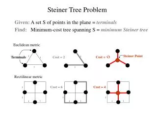
Definition of Steiner tree-(1) Given a graph G=(V,E), a subset RV of vertices, and a length function d:E+ on the edges, a steiner tree is a connected and acyclic subgraph of G which spans all vertices of R
Definition of Steiner tree-(2) • The vertices in R are usually referred as terminals and vertices in V\R as steiner (or optional) vertices • Note that a steiner tree might contain the steiner vertices. The length of a steiner tree is defined to be the sum of the lengths of all its edges • The so-called steiner tree problem is to find a steiner minimum tree, i.e., steiner tree of minimum length • Please see Fig 1
5 6 5 2 2 2 3 3 4 2 2 4 13 Fig 1
Applications & Hardness • Applications: VLSI design, network routing, wireless communications, computational biology • The problem is well known to be NP-complete [R.M. Karp, 1972], even in Euclidean metric or rectilinear metric
Definition of Steiner tree Approximation Algorithms Definition of full Steiner tree A greedyapproximation algorithms ratio3/2, in some special condition ratio8/5,in the worst case Conclusion
Approximation Algorithms • Many important problems are NP-complete or worse • They are approximation algorithms • How good are the approximations ? • We are looking for theoretically guaranteed bounds, not empirical bounds
Some Definitions • Given an optimization problem, each problem instance x has a set of feasible solutions F(x) • Each feasible solution sF(x) has a cost c(s)Z+ • The optimum cost is opt(x)=minsF(x)c(s) for a minimization problem • Its opt(x)=maxsF(x)c(s) for a maximization problem
Approximation Algorithms • Let algorithm M on x returns a feasible solution • M is an -approximation algorithm, where 0, if for all x, • For a minimization problem, • For a maximization problem,
Lower and Upper Bounds • For a minimization problem: • So approximation ratio • For a maximization problem: • So approximation ratio • The above are alternative definitions of -approximation algorithms • between 0 and 1, if P=NP, then =0
Definition of Steiner tree Approximation Algorithms Definition of full Steiner tree A greedyapproximation algorithms ratio3/2, in some special condition ratio8/5,in the worst case Conclusion
Definition of full steiner tree-(1) • A steiner tree is full if all terminals are leaves of the tree • If we restrict the lengths of edges to be either 1 or 2, then the problem is called the (1,2)-full steiner tree problem(FSTP(1,2)) • In order to make sure that a full steiner tree exists, we restrict the given graph G=(V,E) to be complete and R to be a proper subset of V in the FSTP
Definition of full steiner tree-(2) • The length function d is called a metric if it satisfies the following three conditions: • d(x,y)0 for any x, y in V, where equality holds iff x=y • d(x,y)=d(y,x) • d(x,y)d(x,z)+d(z,y) for any x, y, z in V
MIN-FSTP(1,2) • MIN-FSTP(1,2)(minimum (1,2)-full steiner tree problem): Given a complete graph G=(V,E) with a length function d: E+ on the edges and a proper subset RV of terminals, find a full steiner tree of minimum length in G
Applications & Hardness • Applications: Phylogenetic tree (evolutionary tree), telephone communication • Please Fig 2 • FSTP and FSTP(1,2) are NP-complete • In this paper, we give a 8/5 approximation algorithm for the FSTP(1,2)
Definition of Steiner tree Approximation Algorithms Definition of full Steiner tree A greedyapproximation algorithms ratio3/2, in some special condition ratio8/5,in the worst case Conclusion
Some important properties • Let steiner star be a star with a steiner vertex as its center() and the terminals as its leaves(), where center() and leaves() denote the center and the leaves of , respectively • For a steiner star with |leaves()|2, we define its average length f() as follows: • For convenience, we use k-star to denote a steiner star with k leaves and d(center(),v)=1 for each v of leaves ()
Some important lemmas-(1) • Lemma 1: Let be a steiner star with k terminals, where k2. If contains no leaf at distance 1 from center(), then f()=2+2/(k-1) • Lemma 2: Let be a steiner star with k terminals, where k2. If contains only one leaf at distance 1 from center(), then f()=2+1/(k-1) • Lemma 3: Let be a steiner star with k terminals, where k2. If contains exactly two leaves at distance 1 from center(), then f()=2
Some important lemmas-(2) • Lemma 4: Let be a xk-star with k3. Then f()=1+1/(k-1) • Lemma 5: Let 1 be an xk-star with k3 and let 2 be the steiner star obtained from 1 by adding a new terminal z with d(center(1),z)=2. Then f(2)>f(1)
APX-FSTP(1,2)-(1) • Input: A complete graph G=(V,E) with d:E{1,2} and a set RV of terminals • Output: A full Steiner tree APX for R in G • Step 1: Let be an empty set • Step 2: /* Choose a steiner tree with the minimum average length */ • if there are two or more remaining steiner vertices then find a steiner star with the minimum average length; • if f()=2 then /*Transform into an 2-star*/ • Remove from those leaves at distance 2 from center() • end if • else Let be the steiner star with the only steiner vertex as its center and remaining terminals as its leaves
APX-FSTP(1,2) • Step 3:/*Perform a reduction*/ • Let ={(center(),v)|vleaves()} • Replace the steiner star by a single new terminal, say z; • Let d(z,u)=d(center(),v) for each remaining vertex u; • Step 4: • if there is still more than one terminal then go to step 2; • else let APX be the full steiner tree induced by ; • end if
Define of Steiner tree Approximation Algorithms Define of full Steiner tree A greedyapproximation algorithms ratio3/2, in some special condition ratio8/5,in the worst case Conclusion
A 3/2 analysis-(1) • Let the performance ratio of APX-FSTP(1,2) for instance I be ratio(I)=APX(I)/OPT(I) • In the following, we assume that I is a worst-case instance among all instances. That is, ratio(I’)ratio(I) for each I’I
A 3/2 analysis-(2) • Lemma 6: If instance I contains an k-star for k6, then ratio(I)3/2 • Let be an arbitrary k-star whose k is maximum and let E() be the set of its edges • By lemma 1~5, the first iteration of APX-FSTP(1,2) will reduce first • Let I’ be the resulting instance of APX-FSTP(1,2) after is reduced • Clearly, APX(I’)=APX(I)-k
A 3/2 analysis-(3) • Let OPT be an optimal full steiner tree of I, and let ☺be the resulting graph obtained by adding the k edges of E() to • Then by removing from ☺ some edges not in E() and adding one edge if possible, we can build a full steiner tree ’ of I such that it contains all edges of E() • Fig 3 illustrate the worst case
{OPT+E()}-{some edges not in E()}+(center(),v)= full steiner tree ’ contains E() for I OPT v ’ center() Fig 3
A 3/2 analysis-(4) • Clearly, the length of ’ is less than or equal to OPT()+2 since d(center(),v)2 • If we reduce in ’, then we obtain a full steiner tree ’’ of instance I’ whose length is less than or equal to OPT(I)-k+2 • In other words, OPT(’’)OPT(I)-k+2
A 3/2 analysis-(5) • Hence, ratio(I’)=APX(I’)/OPT(I’)(APX(I)-k)/(OPT(I)-k+2) • Recall that ratio(I’)ratio(I) • Hence, we have ratio(I)3/2
Questions and Discuss • Why f() divides |leaves()|-1 ? not |leaves()| ? • Because divides |leaves()| will let APX-FSTP(1,2) fails • Is APX-FSTP(1,2) suits for FSTP(, 2) ? • By lemma 6, it seems ok • What is the case FSTP(1,2,3) ?
The Full Steiner tree problemPart Two Reporter: Cheng-Chung Li2004/07/05
Outline • The 8/5 ratio analysis • Hardness
Some properties • In the following, we assume instance I contains no such an k-star with k 6 and we will then show that ratio(I)8/5 • Given an instance I consisting of G=(V,E) and RV, we say that vertex vV 1-dominates (or dominates for simplicity) itself and all other vertices at distance 1 from v • For any DV, we call it as 1-dominating set( or dominating set) of R if every terminal in R is dominated by at least one vertex of D • A dominating set of R with minimum cardinality is called as a minimum dominating set of R
Lemma 7 • Lemma 7: Given an instance of MIN-FSTP(1,2), let D be a minimum dominating set of R. Then OPT(I)n+|D|-1, where n=|R| …
Some Definitions • Let D be a minimum dominating set of R • We partition R into many subsets in a way as follows: Assign each terminal z of R to a member of D which dominates it • If two or more vertices of D dominate z, then we arbitrarily assign z to one of them • Let Ψ1, Ψ2, …Ψq be the partition consisting of exactly 5 terminals, clearly, we have 0qn/5
Lemma 8 • Lemma 8: OPT(I)5n/4 – q/4 – 1 • According to the partition of R, we have 5q+4(|D|-q)n, which means that |D|(n-q)/4 • Recall that OPT(I)n+|D|-1, then because |D|(n-q)/4 OPT(I)5n/4 – q/4 – 1
Lemma 9-(1) • Lemma 9: If instance I contains no k-star with k6, then ratio(I)8/5 • Assume that FSTP(1,2) totally reduces j ki-stars, where 1ij • Even though the instance I contains no k-star with k6, the reduced k-star may be x6 for i2 • However, it’s impossible that ki-star is an xk-star with k7
Lemma 9-(3) • Note that ki is a subtree of the full steiner tree APX produced by APX-FSTP(1,2) and its length is ki • Since the reduction of ki merges ki old terminals into a new one, the number of the terminals is decreased by ki-1 • After reduced xkj, the number of remaining terminals is • To reduce these terminals, APX-FSTP(1,2) creates a steiner star with length less than or equal to 2
Lemma 9-(4) • Hence , the total length of APX is less then of equal to • In other words, we have APX(I)2n-p, where we let
Lemma 9-(5) • Next, we claim that p11q/10 • The best situation is that each partition Ψi, where 1iq, corresponds to an kl-star, where 1lj, and kl=5 or 6, which will be reduced by APX-FSTP(1,2) • In the case, each such an kl-star contributes at least 3 to p and hence we have p3q> 11q/10
Lemma 9-(6) • Otherwise, we consider the general case with the following five properties, where for simplicity of illustration, we assume that q2=0 (mod 2), q3=0(mod 3), q4=0(mod 4), q5=0(mod 5), and q1+q2+…+q5=q • There are q1 partitions Ψi1,Ψi2,…Ψiq1, in which each partition Ψih,corresponds to an kl-star reduced by APX-FSTP(1,2), where 1hq1
Lemma 9-(10) • There are q2 partitions Ψiq1+1,Ψq1+2,…Ψiq1+q2, in which every other two consecutive partitions Ψiq1+h+1 and Ψiq1+h+2 corresponds to an kl-star reduced by APX-FSTP(1,2), where 1hq2-2 and h=0(mod 2) • … • There are q5 partitions Ψiq1+q2+q3+q4+1,Ψq1+q2+q3+q4+2,…Ψiq1+q2+q3+q4+q5, in which every other five consecutive partitions Ψiq1+q2+q3+q4+h+1 and Ψiq1+q2+q3+q4+h+2, … Ψiq1+q2+q3+q4+h+5 corresponds to an kl-star reduced by APX-FSTP(1,2), where 1hq5-5 and h=0(mod 5)
Lemma 9-(11) • It is not hard to see that the reduction of kl-stars of property(1)(respectively, (2)-(5)) will contribute at least 3q1(respectively, 3q2/2, 3q3/3, 3q4/4, 3q5/5) to p and in the worst case, produce 0(respectively, q2/2, 0, q4/4, and 0) 3-star and produce 0(respectively, 0, 2q3/3, 3q4/4 and 5q5/5)4-star in the remaining instance • In the worst case, the (0+q2/2+0+q4/4+0=(2q2+q4)/4) produced 3-stars and the (0+0+2q3/3+3q4/4+5q5/5=(8q3+9q4+12q5)/12) produced 4-stars will further contribute 1((2q2+q4)/4)/3 and 2((8q3+9q4+12q5)/12)/4, respectively to p
Lemma 9-(12) • Hence, we have • pq1+264q/24011q/10 • If q16/7(n80/7), the ratio(I)8/5 • If n<80/7, the optimal solution can be found by an exhaustive search in polynomial time
Some definitions-(1) • Given two optimization problem 1 and 2, we say that 1 L-reduces to 2 if there are polynomial-time algorithms f and g and positive constant and such that for any instance I of 1, the following conditions are satisfied: • Algorithm f produces an instance f(I) of 2 such that OPT(f(I))OPT(I), where OPT(I) and OPT(f(I)) stand for the optimal solutions of I and f(I), respectively • Given any solution of f(I) with cost c2, algorithm g produces a solution of I with cost c1 in polynomial time such that |c1-OPT(I)||c2-OPT(f(I))|
Some definitions-(2) • A problem is said to be MAX SNP-hard if a MAX SNP-hard can be L-reduced to it • P=NP if any MAX SNP-hard problem has a PTAS • A problem has a PTAS(polynomial time approximation scheme) if for any fixed >0, the problem can be approximated within a factor of 1+ in polynomial time • On the other hand, if 1 L-reduces to 2 and 2 has a PTAS, then 1 has a PTAS
Hardness-(1) • We will show that the optimization problem of FSTP(1,2), referred to as MIN-FSTP(1,2), is MAX SNP-hard by an L-reduction from the vertex cover-B problem • From the proof of this MAX SNP-hardness, it can be easy to see that the decision problem FSTP(1,2) is NP-hard