Download
1 / 33
330 likes | 426 Views
Stochastic Steiner Tree without a Root. Martin P ál Joint work with Anupam Gupta. Steiner Tree. Input : graph G , weights c e on edges, set of terminals g = { t 1 , t 2 , …, t n }. Solution : a network connecting all terminals. Goal : minimize cost of the network built.

E N D
Stochastic Steiner Tree without a Root Martin Pál Joint work with Anupam Gupta Stochastic Steiner without a Root
Steiner Tree Input: graph G, weights ce on edges, set of terminals g = {t1, t2, …, tn} Solution: a network connecting all terminals. Goal: minimize cost of the network built. Note: optimal network will be a tree. Stochastic Steiner without a Root
Stochastic Steiner tree What if the terminals are not known beforehand? ? Installing edges in advance reduces cost – but planning must be done obliviously. We may not be able to correctly connect all demands – but hopefully we will be allowed to fix things later by buying extra edges. ? ? ? ? ? Stochastic Steiner without a Root
drawn from a known distribution π The model Two stage stochastic model with recourse: On Monday, edges are cheap, but we do not know the set of terminals. We can buy edges. On Tuesday, set g of terminals materializes. We must buy edges to connect up g. Edges are σ times more expensive. (σ == inflation factor). Stochastic Steiner without a Root
Want compact representation of F2 by an algorithm The model Two stage stochastic model with recourse: Find F1 Edges and F2 : 2Users 2Edges to minimize cost(F1) + σ Eπ(g)[cost(F2(g))] subject to connected(g, F1 F2(g)) for all sets gUsers Stochastic Steiner without a Root
First stage not connected subgraph Two distant groups Pr[] = Pr[] = ½ σ > 2 Two nearby groups Stochastic Steiner without a Root
The Rent or Buy problem (1) Input: graph G, weights ce on edges, set of demand pairs D,a constant M≥1 Solution: a set of paths, one for each (si,ti) pair. Goal: minimize cost of the network built. Stochastic Steiner without a Root
Steiner forest: pay ce for every edge used The Rent or Buy problem (2) Rent or buy: Must rent or buy each edge. rent: pay ce for each path using edge e buy: pay Mce Goal: minimize rental+buying costs. Stochastic Steiner without a Root
Rent or Buy as Stochastic Steiner Let gi ={si,ti} π(gi) = 1/n σ = M/n install e in first stage buy einstall e in second stage rent e Stochastic Steiner = generalized RoB Each group gi has tree Ti (may have exponentially many groups) Stochastic Steiner without a Root
The Algorithm 1. Boosted Sampling: Draw σ groups of clients g1,g2,…,gσ indep. from the distribution π. • Build a Steiner forest F1 on {g1,g2,…,gσ} using an -approx algorithm. 3. When actual group g of terminals appears, build a tree spanning g in G/F1. Stochastic Steiner without a Root
Bounding the cost Expected first stage cost is small: Lemma: There is a forest F on sampled groups with E[cost(F)] OPT. e installed in first stage OPT: Pr[e is in F] = 1 e not in first stage OPT: Pr[e is in F] ≤ σ Pr[e is in some Ti] Using -approx, can get OPT Theorem: Expected cost of bought edges is OPT. Stochastic Steiner without a Root
pays rent pays buy pays buy pays rent pays rent pays buy Bounding the second stage cost Unselected groups pay their rental cost Selected groups contribute towards buying its tree Plan: Bound second stage cost by the first stage cost: Expected second stage() Expected share() Stochastic Steiner without a Root
Need a cost sharing algorithm Input: Set of demand groups S Output: Steiner forest FS on S cost share ξ(S,g) of each group gS Set of demands demand group ξ({}, ) = 4 ξ({}, ) = 5 Stochastic Steiner without a Root
Rental of if FS bought of share if added to S Cost Sharing for Steiner Forest (P1) Good approximation:cost(FS) St*(S) (P2) Cost shares do not overpay: gSξ(S,g) St*(S) (P3) Strictness: let S’ = S {g}MST(g) in G/ FS ξ(S’,g) Example: S = {} g = Stochastic Steiner without a Root
Bounding second stage cost S’ = {g1,g2,…,gσ} and S = S’– {}.Imagine Pr[S’ | S] = σ π(). E[rent() | S] π()σMST() in G/FS E[rent()] E[buy()] E[buy() | S] = π()σ ξ(S+,) jD E[rent(j)] jD E[buy(j)] OPT Stochastic Steiner without a Root
Computing shares using the AKR-GW algorithm ξ(): ξ(): ξ(): Active terminals share cost of growth evenly. Stochastic Steiner without a Root
1 1+ε 1 AKR-GW is not enough cost share() = 1/n + rental() = 1 + Problem: cost shares do not pay enough! Solution: Force the algorithm to buy the middle edge - need to be careful not to pay too much Stochastic Steiner without a Root
1 1+ε 1 Forcing AKR-GW buy more Idea: Inflate the balls! Roughly speaking, multiply each radius by > 1 Stochastic Steiner without a Root
ξ() large ξ() small, can take shortcuts ξ() small, can take shortcuts Why should inflating work? layer: only is contributing layer: terminals other than contributing Stochastic Steiner without a Root
Freezing times The inflated AKR-GW • Run the standard AKR-GW algorithm on S • Note the time Tj when each demand j frozen • Run the algorithm again, with new freezing rule:every demand j deactivated at time Tj for some > 1 Stochastic Steiner without a Root
Freezing times The inflated AKR-GW (2) Freezing times Original AKR-GW Inflated AKR-GW Stochastic Steiner without a Root
Easy facts Fact: Any time t: u and v in the same cluster in Original u and v in the same cluster in Inflated Inflated has at most as many clusters as Original Theorem: Forest constructed by Inflated AKR-GW has cost at most (+1)OPT. Pf: adapted from [GW]. Stochastic Steiner without a Root
Proving strictness • Compare: • Original(S+) (cost shares) • Inflated(S) (the forest we buy) • Need to prove: MST() in G/ FS ξ(S+, ) • Lower bound on ξ(S+, ) : alone() • Original(S+) must have connected terminals. Hence it contains a tree P spanning . Use it to bound MST(). Stochastic Steiner without a Root
Simplifying.. • Let be time when Original(S+) connects terminals. • Terminate Original(S+) at time . • In Inflated(S), freeze each term. j at time min(Tj, ). • Simpler graph H: • Contract all edges that Inflated(S) bought. Call the new graph H. • Run both Original(S+) and Inflated(S) on H. • Note that Inflated(S) on H does not buy any edges! Stochastic Steiner without a Root
Comparing Original(S+) & Inflated(S) Freezing times Original(S+) Inflated(S) Freezing times Stochastic Steiner without a Root
(-1) |Tree| ≤ |Alone| If we can prove: we are done. |Waste| ≤ |Alone| |Duplicates| ≤ |Alone| + |Other| Proof idea Correspondence of other (i.e. non-red) layers: Layer l in Original(S+) Layer l’ inInflated(S) |Tree| = |Alone| + |Other| |Other| ≤ |Tree| + |Duplicates| + |Waste| + |Waste| Stochastic Steiner without a Root
Bounding the Waste Claim: If a layer l contains t, then its corresponding inflated layer l’ also contains some t. Pf: By picture. Original(S+) Inflated(S) The only way of wasting a layer l is when the whole group lies inside l’. Stochastic Steiner without a Root
Bounding the Waste (2) l l’ Stochastic Steiner without a Root
Bounding the Waste (3) l l’ Stochastic Steiner without a Root
Bounding the Duplicates # edges cut = #clusters –1 # intersections = 2 # edges # cuts < 2 #clusters |Alone| + |Other|+|Duplicates| < 2(|Alone| + |Other|) Stochastic Steiner without a Root
Summing up |Tree| ≤ 4/(-2) |Alone| Hence we have +1 approximation algorithm with 4/(-2)-strict cost sharing. Setting =4 we obtain a 5+8=13 approximation. Stochastic Steiner without a Root
The End • No need to know π explicitly (sampling oracle is enough) • Is the ball inflation trick necessary? • Derandomize the sampling algorithm (for π given explicitly). • Get stronger strictness to allow multistage algo Stochastic Steiner without a Root
*** Useful Garbage *** Theorem: Inflated AKR-GW is a 2 approximation. Pf: adopted from [GW]. ≤≥≠∫∏∑√∂∆≈∙ Stochastic Steiner without a Root