Download
1 / 42
420 likes | 549 Views
Statistics of the CMB. From Boltzmann equation of photons to power spectra 2-point statistics on the sphere: ML, quadratic estimators, polarisation-specifics. Outline of the lectures. Boltzmann equation of CMB. FLAT SCLICING GAUGE. NEWTONIAN GAUGE. Homogeneous solution.

E N D
Statistics of the CMB • From Boltzmann equation of photons to power spectra • 2-point statistics on the sphere: ML, quadratic estimators, polarisation-specifics Outline of the lectures
Boltzmann equation of CMB FLAT SCLICING GAUGE NEWTONIAN GAUGE Homogeneous solution Perturbed metric reads Perturbed photon energy-momentum
Boltzmann equation of photons Geodesic parametrization Geodesic equation of particles (interacting gravitationally only) Unperturbed ======== background Homogeneous evolution
Perturbed Boltzmann equation Geodesic equation for the energy, in perturbed metric Boltzmann equation for perturbed distribution, in perturbed background Collisional cross-section is frequency independent: can integrate over frequency: STF TENSORS
SVT, STF, Spherical harmonics… Vector field: potential plus solenoidal: STF tensor of rank 2: Generalization: Fourier space, with k=e3 NORMAL MODES
Thomson scattering term (temperature) COLLISION TERM THOMSON PHASE FUNCTION Energy as seen by observer comoving with baryons/photons fluid
Gauge-invariant phase-space density perturbation Gauge-invariant Boltzmann equation reads (Newtonian gauge)
Temperature hierarchy, scalar modes Monopole is unaffected by scattering Forward photons are scattered away Baryon-photon drag Anisotropic pressure USING THE FOLLOWING GRAVITY THOMSON SCATTERING TRANSPORT
Einstein and conservation equations Scalar modes, Einstein equations Constraint equations (Poisson) Evolution equations Scalar modes, conservation equations Energy Momentum (Euler) Tensor modes, Einstein equation
DO YOU (REALLY) THINK THIS IS IT ?? NOT YET…. POLARISATION OK, I’ll make it soft !
Polarisation • Due to quadrupolar anisotropy in the electron rest frame • Linked to velocity field gradients at recombination
E and B modes of polarisation Scalar quantity Pseudo-scalar quantity Scalar perturbations cannot produce B modes B modes are model-independent tracers of tensor perturbations
Normal modes are gauge-invariant (Stewart-Walker lemma) As for temperature, we have normal modes for polarisation Temperature and polarisation get decomposed on these modes
Boltzmann equation for Stokes Q,U Redefining SIMPLE, ISN’T IT ? Stokes parameters are absent in unperturbed background Their evolution does not couple to metric perturbations at linear order
Polarized scattering term SCATTERING GEOMETRY
Boltzmann polarization hierarchy ONLY E-MODES COUPLE TO TEMPERATURE QUADRUPOLE SCALARS DO NOT PRODUCE B MODES As for the temperature case, express gradient term in terms of spherical harmonics Using the following recurrence formula:
Normal modes and integral solutions Interpretation State of definite total angular momentum results in a weighted sum of SOURCE DEPENDANCE PLANE WAVE MODULATION Using recurrence relations of spherical Bessels: Develop the plane wave into radial modes
Normal modes and integral solutions Linear dependance in the primordial perturbations amplitudes These normal modes are the solutions of the equations of free-streaming !! (Boltzmann equation without gravity and collisions) • Line-of-sight integration codes • Sources depend on monopole, dipole and quadrupole only
CMB power spectra Wayne Hu
CMB imaging: scanning experiments Time-response of the instrument (detector + electronics) Simplified linear model (pixelized sky) EM filters band-pass Detector noise Angular response: beam and scanning strategy BICEP focal plane Spider web bolometer Archeops, Kiruna
Imagers: map-making Huge linear system to solve: use iterative methods (PCG) + FFTs BAYES theorem Linear data model Uniform signal prior Sufficient statistics Covariance matrix of the map
Imagers: power spectrum Signal covariance matrix BAYES again… Marginalize over the map TO BE MAXIMIZED WITH RESPECT TO POWER SPECTRUM
Imagers: power spectrum (cont.) PSEUDO-NEWTON (FISHER) Second order Taylor expansion For each iteration and each band, Npix3 operation scaling !!
Imagers: too many pixels ! Quite ugly at first sight !! New (fast) analysis methods needed • Fast harmonic transforms • Heuristically weighted maps
Imagers (cont.) Power spectrum expectation value …simplifies, after summation over angles (m):
Imagers: “Master” method Finite sky coverage loss of spectral resolution need to regularize inversion Spectral binning of the kernel Unbiased estimator MC estimation of covariance matrix of PS estimates Works also for polarization (easier regularization on correlation function)
Imagers: polarised map-making One polarised detector (i) Let us consider n measurements of the same pixel, indexed by their angle ML solution
Polarisation: optimal configurations General expression of the covariance matrix Assume uncorrelated and equal variance measurements, look for optimal configuration of angles : • Stokes parameters errors are uncorrelated • Covariance determinant is minimized
Imagers: polarised spectrum estimation Stokes parameter in the great circle basis
Polarisation: correlation functions Polynomials in cos(): integrate exactly with Gauss-Legendre quadrature
Polarisation: (fast) CF estimators for m=n=2 involves Using with Weighted polarization field Using We get Heuristic weighting (wP,wT): Normalization: correlation function of the weights
Polarisation: (fast) CF and PS estimators Define the pseudo-Cls estimates: These can be computed using fast SPH transforms in O(npix3/2) (compare to o(npix3) scaling of ML…) If CF measured at all angles: integrate with GL quadrature Assuming parity invariance
Polarisation: CF estimators on finite surveys Results in E/B modes leakage Incomplete measurement of correlation function: apodizing function f(): Normalization of the window functions
Polarisation: E/B coupling of cut-sky Leakage window functions (not normalized) Recovered BB spectra (dots) No correlation function information over max=20±
Polarisation: E/B coupling of cut-sky No correlation function over Gaussian apodization Leakage window functions (not normalized) Recovered BB spectra (dots)
Polarisation: E/B leakage correction Define: Then: We have obtained pure E and B spectra (in the mean) As a function of +
Quadratic estimators: covariances RAPPELS Edge-corrected estimators covariances in terms of pseudo-Cls covariances As long as Mll’ is invertible, same information content in edge-corrected Cls and pseudo-Cls
Pseudo-Cls estimators: cosmic variance Forget noise for the moment, consider signal only: Case of high ells and/or almost full sky If simple weighting (zeros and ones)
The case of interferometers CBI – Atacama desert
Interferometers: data model Visibilities: sample the convolved UV space: Relationship between (Q,U) and (E,B) in UV (flat) space Idem for Q and U Stokes parameters RL and LR baselines give (Q§iU) Visibilities correlation matrix UV coverage of a single pointing of CBI (10 freq. bands) ( Pearson et al. 2003)
Pixelisation in UV/pixel space • Redundant measurements in UV-space • Possibility to compress the data ~w/o loss Use in conjonction with an ML estimator Newton-like iterative maximisation Least squares solution • Hobson and Maisinger 2002 • Myers et al. 2003 • Park et al. 2003 Fisher matrix For an NGP pointing matrix: Covariance derivatives for one visibility Resultant noise matrix