Download
1 / 14
140 likes | 227 Views
Cmad simulation code status Tracking the beam in a MAD lattice, parallel code, interaction with cloud at each element in the ring and with different cloud distribution, single-bunch instability studies, threshold for SEY, dynamic aperture tune shift …

E N D
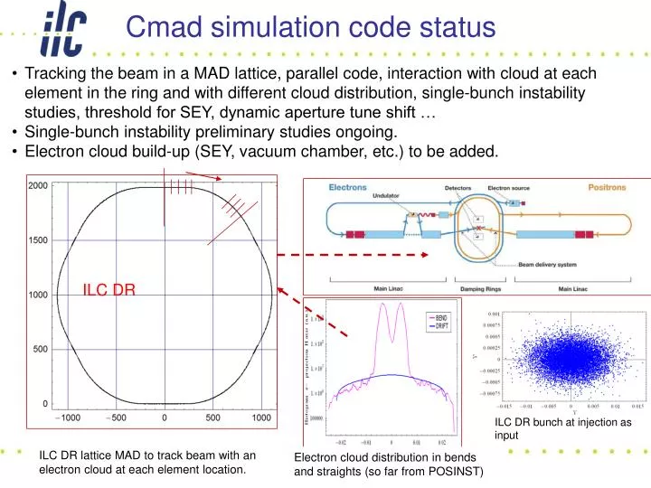
Cmad simulation code status • Tracking the beam in a MAD lattice, parallel code, interaction with cloud at each element in the ring and with different cloud distribution, single-bunch instability studies, threshold for SEY, dynamic aperture tune shift … • Single-bunch instability preliminary studies ongoing. • Electron cloud build-up (SEY, vacuum chamber, etc.) to be added. ILC DR ILC DR bunch at injection as input ILC DR lattice MAD to track beam with an electron cloud at each element location. Electron cloud distribution in bends and straights (so far from POSINST)
Goals • simulate electron cloud instability threshold in the LC DRs, LHC, SPS and storage rings Status • Benchmarked against codes at CERN web page. Good agreement with existing codes (HEAD-TAIL “new simulation results 2006”) for 1 interaction point/turn. Ongoing SPS and ILC DR simulations and code benchmarking. • Beta version, still good room to gain in speed: Electric fields calculation to be upgraded, parallel features to be optimized
Dynamics Beam and electron cloud Dynamics: • MAD sectormap and optics functions files as input • Tracking 1 bunch in the lattice by 1st (switch for 2nd) order transport maps R (and T) • Particle in cell PIC code • Tracking 6D beam phase space, 3D beam dynamics • 3D electron cloud dynamics • Apply beam-cloud interaction at each element of MAD lattice • 2D forces beam-cloud, cloud-cloud computed at interaction point • Electron dynamics: cloud pinching and magnetic fields included
Code benchmarking CMAD with Head-Tail code “new simulation results 2006” on web page. 1 interaction point/turn. CMAD with 32 processors in this simulation on seaborg/nersc IBM6000.
SPS simplified model Emittance growth simulated with TAILHEAD considering a single electron-beam interaction point at the center of each half cell (left) and with two interaction points, close to the QD and QFF quadrupoles (right). The electron cloud responds either dynamically, or it is frozen. The electron density is 2.75e11 m-3 for the left picture and either 1e11 m-3 or 2e11 m-3 on the right. SPS simplified model.
SPS simplified model Emittance growth simulated with CMAD considering a single electron-beam interaction point at the center of each half cell (left) frozen potential after first interaction . The electron density is 2.5e11 m-3 to 7.5e11m-3. SPS simplified model.
Improvements: • Electric field computation is actually a direct node to node (slow) computation and interpolation – Room for improvement here…! • Actually looking into Multigrid parallel like PHAML
Improvements: • Electric field computation is actually a direct node to node (slow) computation and interpolation – Room for improvement here…! • Actually looking into Multigrid Poisson parallel solver like PHAML • Suggestions for improvement?! • Parallel improvement: • Actually computing beam-cloud interaction with all processors for each ring element • Next: assign a ring section of N elements to N processors to each compute beam-cloud interaction, then track the beam through the N elements (assume weak beam changes)
Discussion, ideas, suggestions Approximations to be added: • Optional: If beta functions are identical at two elements in phase (2*pi*n), apply earlier computed cloud-potential Approximations [Longer term!] to be added: • Build-up of the electron cloud initially computed until saturation for each representative of magnet class and density distributed over the ring; Then updated at each turn (assuming weak changes of the beam turn by turn).. Improvements [to be added?!]: • Symplectic integrators tracking: needed ? (but ~98% phase space conserved with R and T tracking, ILCdr 1000 turns)
!**************************************** • ! SET UP PARALLEL COMPUTATION • ! *************************************** • CALL MPI_INIT(ierror) ; ! Initialize MPI • CALL MPI_COMM_SIZE(MPI_COMM_WORLD, numTasks, ierror); ! Find number of Tasks (processors) • CALL MPI_COMM_RANK(MPI_COMM_WORLD, me , ierror); ! Find the ID of this task • ! ****************************** • ! *** START MAIN LOOP ***** • ! ****************************** • CALL READ_INPUT_FILES ! READ 1) input file 2) IF(me==0) CALL BEAM_GENERATE ! GENERATE PARTICLES BEAM • IF(me==0) CALL PRINT_BEAM_DISTRIBUTION ! PRINT ALL BEAM PARTICLES ON FILE • DO 200 nturn = 1, nturns; • CALL BEAM_DISTRIBUTION ! UPLOAD AND ORDER LONGITUDINALLY-SLICED BEAM DISTRIBUTION • CALL PARTITION_BEAM_PARTICLES ! PREPARE TO ASSIGN BEAM PARTICLES TO EACH PROCESSOR • CALL MPI_BCAST(xxx, count, MPI_REAL, root, MPI_COMM_WORLD, ierr) ; ! PROCESSOR 0 PASSES THE PARTICLE BEAM • DO 100 ielement = 1, NumberOfElements ! LOOP OVER NumberOfElements = TOTAL NUMBER OF NON-ZERO ELEMENTs • CALL GRID_SETUP(ielement) ; • CALL REMOVE_PARTICLES_EXCEEDING_APERTURE(ielement) • IF(justtrackbeam==1) then; CALL BEAM_TRACK_PARALLEL(ielement,ielement); goto 75; endif; ! TRACK BEAM WITHOUT CLOUD • IF( ELENGHT(ielement) == 0.0 .and. nturn > 1) goto 70 ! SKIP ZERO-LENGTH ELEMENTS • IF(ifrozen==1 .and. nturn > 1) then; CALL FROZEN_ELECTRIC_FIELD(ielement,frozen3Dcloud) ; goto 70; endif; • CALL BEAM_ON_3DGRID(ielement,grid3Dbeam) • CALL ELECTRON_CLOUD_DISTRIBUTION(ielement) • CALL PARTITION_ELECTRON_CLOUD ; countel = nemax * 6 ; • CALL MPI_BCAST(xxxel, countel, MPI_REAL, root, MPI_COMM_WORLD, ierr); ! PROCESSOR 0 PASSES THE PARTICLE • CALL ELECTRIC_FIELD(ielement,grid3Dbeam,grid2Dcloud,frozen3Dcloud) ; • 70 CONTINUE • CALL BEAM_TRACK_PARALLEL(ielement,ielement); • 75 CONTINUE • ! *** PROCESSOR me=0 GATHER XXX BACK FROM ALL PROCESSORS *** • !!!!!!!!!!! THIS IS SLOW IMPROOVE HERE !!!!!!! … (more lines cut) • CALL MPI_SEND(xxxsend, isendcount, MPI_REAL, root, itag, MPI_COMM_WORLD, ierr) • CALL MPI_RECV(xxxrecv, iksendcount, MPI_REAL, k, itag, MPI_COMM_WORLD, istatus, ierr) • !!!!!!!!!!! THIS IS SLOW IMPROOVE HERE !!!!!!! END • CALL FLUSH_OUT • DEALLOCATE(grid3dbeam,grid2dcloud) • 100 CONTINUE • IF(me==0) CALL PRINT_BEAM_DISTRIBUTION • IF(me==0) CALL SYNCHROTRON_OSCILLATION • 200 CONTINUE • CALL COMPUTE_AND_PRINT_BEAM_STATISTICS(ielement-1, numfile); ! print on a file the standard deviations • CALL close_files • ! ****************************** • ! **** END MAIN LOOP **** • !*******************************
SPS simplified model: synchrotron oscillations. synchrotron tune Qs=0.0025.