SEM PURPOSE

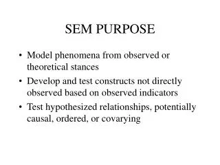
1. SEM PURPOSE • Model phenomena from observed or theoretical stances • Develop and test constructs not directly observed based on observed indicators • Test hypothesized relationships, potentially causal, ordered, or covarying

2. Relationships to other quantitative methods

3. Decomposition of Covariance/Correlation • Most hypotheses about relationship can be represented in a covariance matrix or set of matrices • SEM is designed to reproduce the observed covariance matrix as closely as possible • How well the observed matrix is fitted by the hypothesized matrix is Goodness of Fit • Modeling can be either entirely theoretical or a combination of theory and revision based on imperfect fit of some parts.

4. Decomposition of Covariance Matrix Consider a covariance matrix of observed variables: y1 y2 x1 x2 y1 1 .6 .5 .6 y2 .6 1 .3 .2 S = x1 .5 .3 1 .4 x2 .6 .2 .4 1 Suppose each correlation could be “taken apart” or decomposed into parts associated with relationships among the variables for a specific model:

5. THEORETICAL MODEL BY RESEARCHER Example: Age (X1) and Letter naming (X2) predict Word identification (Y1), and all predict Simple Reading Comprehension (Y2). a X1 Y1 r12 b c e X2 d Y2 Define correlation as the sum of “paths from one variable to another. For example r(X1, Y1) = a + r12*c r(X2, Y2) = d + c*b + r12*e r(X1, Y2) = e + a*b + r12*d r12 = Pearson Corr (X1,X2) r(Y1, Y2) = b + c*d r(X2, Y1) = c + r12*a

6. EMPIRICAL ESTIMATES OF PATH COEFFICIENTS .310 X1 Y1 .4 .476 .736 .034 ns X2 -.255 Y2 y1 y2 x1 x2 y1 1 .6 = .736-.476*.255+.310*.034 .5 .6 y2 .6 1 .3 .2 x1 .5 .3 = .034+.31*.736-.4*.255+ .4*.476*.736 1 .4 x2 .6 .2 = -.255+.476*.736+.4*.034+.4*.31*.736 .4 1

7. TERMS X1 and X2 are exogenous (exo=outside, gen= generated) variables: no variables predict them Y1 and Y2 are endogenous (endo=inside) variables; predicted from other variables that may be either exogenous or endogenous

8. JUST-IDENTIFIED MODEL The number of parameters that were fit in the above example was exactly equal to the number of degrees of freedom # exogenous = P # endogenous = Q dftotal = (P+Q)(P+Q+1)/2 In our example df = 4*5/2 = 10

9. JUST-IDENTIFIED MODEL In our example df = 4*5/2 = 10 y1 y2 x1 x2 y1 1 .6 .5 .6 y2 .6 1 .3 .2 S = x1 .5 .3 1 .4 x2 .6 .2 .4 1 4 terms were “constrained”, the 4 variances, leaving 6 df- we don’t estimate the correlation of a variable with itself.

10. JUST-IDENTIFIED MODEL The 5 parameters we estimated, a-e, the path coefficients, were solvable from 5 simultaneous equations. Since we fit the correlation matrix exactly, all degrees of freedom are used

11. UNDER-IDENTIFIED MODEL Suppose we redraw the model to include errors of prediction: e1 a X1 Y1 r12 b c e X2 d Y2 e2 If we hypothesized that the errors were correlated (putting a curved arrow as shown), we would not have sufficient df to estimate the model, so we say the model in under-identified.

12. OVER-IDENTIFIED MODEL If the number of total parameters estimated is less than the df, the model is Over-identified. For example, suppose in our model we assume one path is equal to zero. Since we don’t have to estimate the path, we have a degree of freedom. Over-identified models can be compared to the Just-identified model or to other Over-identified models with more or fewer parameter constraints

13. CONSTRAINING PARAMETERS We can reduce the number of parameters to achieve either Just-Identified or Over-identified model status by fixing paths or variances to specific values. For example, in our model, suppose path e is assumed to be equal to zero. Then we have reduced the model back to just-identified status including the error correlation.

14. JUST-IDENTIFIED MODEL Solving this model is more complex since two new variables, e1 and e2, are now in the model. The solution is: e1 .31 X1 -.061 ns Y1 r12 .846 .476 X2 -.308 Y2 e2 The hypothesized error correlation is not supported in the data. Remember that the path from X1 to Y2 was also not supported. We will discuss modifying our model later.

15. Decomposition of Covariance/Correlation • Under SEM, the following function is computed, termed the fit function F = log  + tr(S-1 ) - logS - (P – Q) • = Hypothesized Covariance matrix specified by our model S = Observed Covariance matrix from the data P = # exogenous variables Q = # endogenous variables

16. Decomposition of Covariance/Correlation • Estimating  becomes the next task after specifying the theoretical model • Estimation methods depend on the assumptions and on data structure and details: • Sample Size • Multicollinearity presence in the data • Variable distributions

17. Developing Theories • Previous research- both model and estimates can be used to create a theoretical basis for comparison with new data • Logical structures- time, variable stability, construct definition can provide order • 1999 reading in grade 3 can affect 2000 reading in grade 4, but not the reverse • Trait anxiety can affect state anxiety, but not the reverse • IQ can affect grade 3 reading, but grade 3 reading is unlikely to alter greatly IQ (although we can think of IQ measurements that are more susceptible to reading than others)

18. Developing Theories • Experimental randomized design- can be part of SEM • What-if- compare competing theories within a data set. Are all equally well explained by the data covariances? • Danger- all just-identified models equally explain all the data (ie. If all degrees of freedom are used, any model reproduces the data equally well) • Parsimony- generally simpler models are preferred; as simple as needed but not simple minded