Download
1 / 124
1.4k likes | 1.89k Views
SRH-1D: Sedimentation and River Hydraulics in One-Dimension. Jianchun Huang, Ph.D., Colorado State University, Fort Collins, CO Blair Greimann, Ph.D., P.E., Technical Service Center, Sedimentation and River Hydraulics Group, Denver, CO Prepared for Taiwan Water Resources Agency, November 2008

E N D
SRH-1D: Sedimentation and River Hydraulics in One-Dimension Jianchun Huang, Ph.D., Colorado State University, Fort Collins, CO Blair Greimann, Ph.D., P.E., Technical Service Center, Sedimentation and River Hydraulics Group, Denver, CO Prepared for Taiwan Water Resources Agency, November 2008 www.usbr.gov/pmts/sediment
What Is SRH-1D ? One – dimensional analysis of: • Unsteady or steady flow • Sediment transport rates • Erosion and deposition
Why SRH-1D? • Why did Reclamation develop SRH-1D? • Full flexibility for research and development • Application to specialized situations • Lack of customizable tools available • We do not try to compete with commercial codes
Reclamation History of Development • 1980s – STARS (Randle) • 1986 – GSTARS (Molinas and Yang) • 1998 – GSTARS2.0 (Yang, Trevino and Simões) • 2000 – GSTARS2.1 (Yang and Simões) • 2003 – GSTARS3 (Yang and Simões) • 2006 – GSTAR-1D 1.1 (Huang and Greimann) • 2007 – SRH-1D V2.0 (Huang and Greimann) • 2008 - SRH-1D V2.1 (Huang and Greimann)
Scales in Modeling • Spatial Scales: • Three-dimensional model (most detailed, smallest scales) • Two-dimensional model (depth-averaged or laterally averaged) • One-dimensional model (cross-sectional averaged) • Time Scales: • Short term: Event based • Long term simulation
SRH-1D Methods • 1D hydraulic model • Single channels and channel networks • Steady and unsteady hydraulic and sediment transport models • Cohesive and non-cohesive sediment transport • Large spatial scale application and long term simulation
Major Features (1/2) • Flow Regimes • subcritical flow computation for steady flow • subcritical, critical, and supercritical flow computation for unsteady flow • Network • simple channel, simple channel network, and complex channel network • Cohesive and non-cohesive sediment transport • cohesive sediment aggregation, deposition, erosion, and consolidation • many sediment transport equations for non-cohesive sediment • Different sediment size fractions • separate routing of different size fractions to simulate sorting and armoring
Major Features (2/2) • Floodplains • separate subchannels for main channel and floodplains, exchange of water and sediment between main channel and floodplains • Point and non-point sources • allowing lateral flow and sediment input from tributary and water shield • Internal boundary conditions • time-stage table, rating curve, weir, bridge, and radial gate • Ability to model channel incision • Erosion width concept for dam removal • Bedrock scour capability
Limits of Application • SRH-1D is a 1D model. It should not be applied to situations where a truly 2D or truly 3D model is needed for detailed simulation of local conditions. • The phenomena of transverse variation of shear stress, transverse sediment movement, secondary currents, diffusion, and super elevation are ignored.
Limits of Application 1D Problem areas: • Lateral sorting (a cross section may armor or degrade faster than predicted) • Pool-riffle sequences (pools fill up and are not scoured) • Changes in plan form (e.g. cannot simulate transitions from braided to meandering) • Bank erosion (hydraulics are not resolved adequately to predict bank erosion)
Limits of Application • General sediment transport modeling problems: • Transport and mixing of gravel-sand mixtures • Sediment supply prediction • Unknown channel modifications • Cohesive sediment • Natural systems are complex and can have high degree of spatial and temporal variability • Each river will have unique qualities • Each river will require judicious application
Steady Flow Computation Energy equation for steady gradually varied flow where z = water surface elevation b = velocity distribution coefficients V = flow velocity hf= friction loss hc = contraction or expansion losses K = conveyance computed from Manning’s equation
Steady Flow Computation-Network • The energy equation and the continuity equation • Upstream B.C. • Downstream B.C. • Final equation:
Steady Flow Computation-Network • Example: • Downstream B.C. for River 1: • Upstream B.C. for River 2: • Upstream B.C. for River 3: • Final equation:
Unsteady Flow Computation de St Venant equations Continuity: Momentum: where Q = discharge (m3/s), A = cross section area (m2), Ad = ineffective cross section area (m2), qlat = lateral inflow per unit length of channel (m2/s), t = time independent variable (s), x = spatial independent variable (m), b = velocity distribution coefficients, Z = water surface elevation (m), and Sf = energy slope
Unsteady Flow Computation • Discretized grid for unsteady flow simulation • Discretized equations
Internal Boundary Conditions • Time Stage Table • Rating Curve • Weir • Bridge • Radial Gate
Sediment Computation • Conceptual model
Sediment Computation • Mass Balance: XC i-1 XC i XC i+1 Water column Qs,i-1 Qs,i+1 Qs,i Se,i Active Layer Sub-Layer
Sediment Computation • Non-Cohesive Sediment Transport Capacity Functions
Cohesive Sediment Physical processes Aggregation Deposition Partial deposition Full deposition Sediment Computation • Erosion • Surface erosion • Mass erosion • Consolidation Erosion Aggregation
Uniform Sediment or Non-Uniform Sediment Model • A uniform model uses a representative particle size for sediment routing. • A non-uniform model routes sediment by size fraction to more realistically reflect the phenomenon of sediment sorting and the formation and destruction of an armor layer on a river bed. • SRH-1D is non-uniform model
Non-equilibrium routing • Equilibrium Model: there is an instantaneous exchange between suspended and bed sediments when there is a difference between sediment supply and a river’s sediment transport capacity • For fine sediments, there is usually a time lag. SRH-1D provides a non-equilibrium model (based on Han, 1990) which takes this phenomenon into consideration
Steady Routing Model Assumptions • Change in suspended sediment concentration at a cross section is much smaller than change of a river bed, i.e., • During a time step, parameters for a cross section remain constant (This allows decoupling of water and sediment computations)
Unsteady Sediment Model • The convection-diffusion equation for unsteady sediment transport: Unsteady Convective Diffusion Source Term Term Term Term
Non-equilibrium Sediment Transport Parameters Suspended Load Bed Load Ltot = total adaptation length qtot = transport capacity b = relative sediment velocity Vt = unit flow discharge h = flow depth C = sediment concentration f = faction of suspended sediment ws = sediment fall velocity a, z = user specified constants
Bed Sorting and Armoring • SRH-1D computes sediment transport by size fraction; it will show particles of different sizes being transported at different rates. Some particle sizes may be eroded, while others may be deposited or may be immovable • SRH-1D computes the carrying capacity for each size fraction present in the bed, but the amount of material actually moved is computed by the sediment routing equation. Consequently, sorting and armoring are simulated
Bed Sorting and Armoring • Kinematic condition • Volume-conservation equation
Channel Width Changes • SRH-1D channel geometry adjustments can be vertical or lateral Vertical adjustment Lateral adjustment Most often, the difference between such adjustments is minor
Channel Side Slope Computation • SRH-1D can check whether the angle of repose exceeds a known critical slope. A user is allowed the option of specifying one critical angle above the water surface, and a different critical angle for submerged points. • SRH-1D scans each cross section at the end of each time step to determine if any vertical or horizontal adjustments have caused the banks to become too steep. • Bank erosion is added as lateral inflow.
Channel Incision • SRH-1D uses an equation related to flow rate to determine erosion width: Erosion Width = a Qb a and b are user defined. • The erosion width can be much smaller than the wetted width (e.g. delta erosion during dam removal
Previous Test and Applications • Simulation of Networks • Canal Sedimentation (San Luis Canal) • Dam Removal (Matilija Dam Removal) • Reservoir Sediment Management (Black Canyon Diversion Dam) • River Restoration (Rio Grande, Trinity River) • River Aggradation for Flood Protection (Little Colorado River)
Running SRH-1D • Click on SRH-1D executable and type in input file. • Command Line: PATH\SRH-1D V2.0.5.EXE inputfile.srh (Optional argument -e to exit window upon completion) • Batch File: set PRG_NM1="..\..\CurrentVersion\SRH-1D V2.0.5.EXE" for %%f in (*.srh) do %PRG_NM1% -e "%%f"
Output Files • sample_OUT.dat: echo of output • sample_ERR.dat: Error file • sample_HEC_RAS_GEOMETRY.g01: HEC-RAS geometry file of current geometry • sample_OUT_Profile.dat: profile information, average cross sectional values • sample_OUT_XC.dat: cross section information • sample_OUT_MaterialVolume.dat: cumulative material volume of deposition
Output Files • sample_OUT_Volume.dat: cumulative volume of deposition material • sample_OUT_MassBalance.dat: mass balance file • sample_OUT_Conc.dat: sediment concentration • sample_OUT_BedLayer.dat: bed thickness data of each bed layer • sample_OUT_BedLayer.dat: bed thickness data of each bed layer
Output Files • sample_OUT_BedFraction.dat: sediment size fraction data of each bed layer • sample_OUT_Porosity.dat: sediment porosity data of each bed layer in each sub-channel. • sample_OUT_SedimentLoad.dat: sediment load passing each cross section • sample_OUT_TimeSeries.dat: time series information at the cross sections • sample_solu.wrt: hot start file
Output Files: Example # output bed profile # t = time(hr) # riv = river number # xc = cross section number # idxc = original cross seciton number # xt = cross section location (ft or m) # q = discharge (cfs or m^3/s) # qlatf = lateral flow discharge (cfs or m^3/s) # zb = current thalweg elevation (ft or m) # z = current water surface elevation (ft or m) # zba = average bed elevation of the main channel (ft or m) # fslope = friction slope (-) # topw = top width (ft or m) # hydrad = hydraulic radius (ft or m) # vel = average velocity for xc (ft/s or m/s) # d16 = sediment size d16 in bed layer 1 (mm) # d50 = sediment size d50 in bed layer 1 (mm) # d84 = sediment size d84 in bed layer 1 (mm) TITLE="bed profile" VARIABLES=t,riv,xc,idxc,xt,q,qlatf,zb,z,zba,fslope,topw,hydrad,vel,d16,d50,d84 0.00000000 1 1 1 5000.00000 14900.0000 0.00000000 1005.00000 … 0.00000000 1 2 #### 4500.00000 14900.0000 0.00000000 1004.50000 … 0.00000000 1 3 #### 4000.00000 14900.0000 0.00000000 1004.00000 …
Examples • Network simulations • Unsteady canal flow and sedimentation • Dam removal impacts in cobble bed river • Sediment sluicing • Long term aggradation and degradation in sand bed channel
1. Network Simulation Simulation of a simple network channel with sediment transport. The network is composed of 4 trapezoidal channels. Rivers are numbered ascending from upstream to downstream
Simulation of a simple network channel with sediment transport. Bed elevation and water surface elevation
2. San Luis Canal (SLC), a reach of the California Aqueduct, extends 75 miles from Check Structure 15 to Check Structure 21
A reach of the California Aqueduct, or San Luis Canal (SLC), extends 75 miles from Check Structure 15 to Check Structure 21 Bed elevation change of the SLC before and after a flood event
A reach of the California Aqueduct, or San Luis Canal (SLC), extends 75 miles from Check Structure 15 to Check Structure 21
3. Matilija Dam Removal • Matilija Dam is located on the Ventura River and now has only 500 ac-ft left of its original 7000 ac-ft capacity • SRH-1D is being used to quantify downstream impacts associated with dam removal • It is being used to predict: sediment concentrations, river bed aggradation, sediment inputs to diversion, sediment delivery to ocean, reservoir erosion