Download
1 / 19

E N D
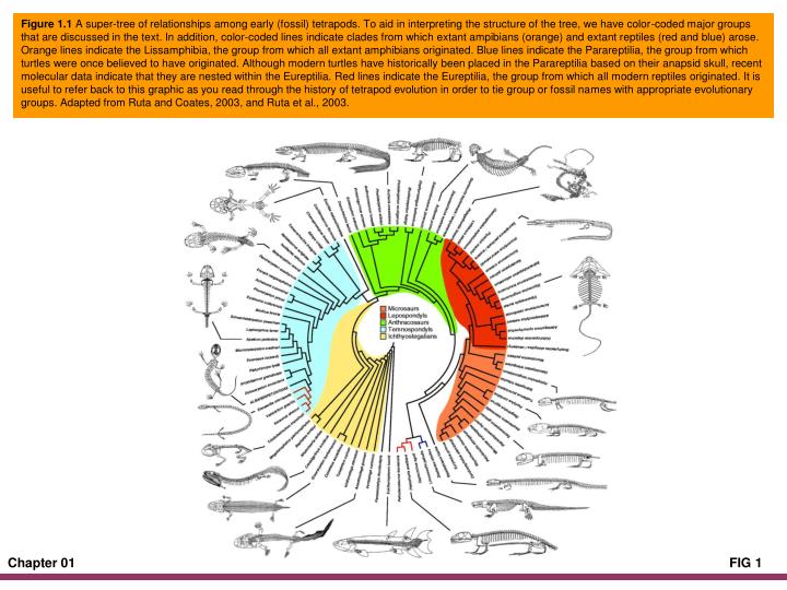
Figure 1.1 A super-tree of relationships among early (fossil) tetrapods. To aid in interpreting the structure of the tree, we have color-coded major groups that are discussed in the text. In addition, color-coded lines indicate clades from which extant ampibians (orange) and extant reptiles (red and blue) arose. Orange lines indicate the Lissamphibia, the group from which all extant amphibians originated. Blue lines indicate the Parareptilia, the group from which turtles were once believed to have originated. Although modern turtles have historically been placed in the Parareptilia based on their anapsid skull, recent molecular data indicate that they are nested within the Eureptilia. Red lines indicate the Eureptilia, the group from which all modern reptiles originated. It is useful to refer back to this graphic as you read through the history of tetrapod evolution in order to tie group or fossil names with appropriate evolutionary groups. Adapted from Ruta and Coates, 2003, and Ruta et al., 2003.
Figure 1.2 A sampling of adult body forms in living amphibians.
Figure 1.3 A sampling of adult body forms in living reptiles.
Figure 1.4 Relationships, body forms, and limb structure of the seven key fossil vertebrates used to recover the evolution of supportive limbs in tetrapods. Glyptolepis is the outgroup. Adapted from Ahlberg and Clack, 2006; Clack 2006; Daeschler et al., 2006; and Schubin et al., 2006.
Figure 1.5 Air-breathing cycle of the longnosed gar (Lepisosteus osseus). As the gar approaches the surface at an angle, it drops its buccal floor and opens its glottis so air can escape from the lungs (bottom center, clockwise). By depressing the buccal floor, the gar flushes additional air from the opercular chamber. Once flushed, the gar extends its snout further out of the water, opens its mouth, depresses the buccal floor drawing air into the buccal cavity, and shuts the opercula. The mouth remains open and the floor is depressed further; then closing its mouth, the gar sinks below the surface. Air is pumped into the lungs by elevating the buccal floor. Adapted from Smatresk, 1994.
Figure 1.6 Fin and limb skeletons of some representative fishes and tetrapods. Top to bottom, ray-finned or actinopterygian fin, osteolepiform lobed fin, actinistian lobed fin, porolepiform lobed fin, lungfish or dipnoan lobed fin, and a tetrapod limb. Adapted from Schultze, 1991.
Figure 1.7 Comparison of the skulls of an early amphibian Edops and an early reptile Paleothyris. Scale: bar = 1 cm. Reproduced, with permission, from Museum of Comparative Zoology, Harvard University
Figure 1.8 A branching diagram of the evolution within the Tetrapoda, based on sister group relationships. The diagram has no time axis, and each name represents a formal clade-group name. After Clack, 1998; Gauthier et al., 1988a,b, 1989; and Lombard and Sumida, 1992; a strikingly different pattern is suggested by Laurin and Reisz, 1997.
Figure 1.9 A branching diagram of the evolution of basal Amniota and early reptiles, based on sister group relationships. The diagram has no time axis, and each capitalized name represents a formal clade-group name. Opinion varies on whether the mesosaurs are members of the Reptilia clade or the sister group of Reptilia. If the latter hypothesis is accepted, the Mesosauria and Reptilia comprise the Sauropsida. Turtles (Testudines) are shown here as nested within the Parareptilia based on morphology. More recent molecular analyses indicate that they are nested in the Eureptilia (see Chapter 18). After Gauthier et al., 1989; Laurin and Reisz, 1995; and Lee, 1997; a strikingly different pattern is suggested by deBraga and Rieppel, 1997.
Figure 1.10 Presence of the amnion defines the Amniota. Viviparity is not necessarily associated with presence of an amnion. This distribution of egg-retention based on extant species does not permit the identification of the condition in basal amniotes. The origin of terrestrial amniotic eggs as an intermediate stage is equally parsimonious with the evolution of amniotic eggs within the oviduct to facilitate extended egg retention. After Laurin and Reisz, 1997.
Figure 1.11 A branching diagram of the evolution of basal reptile clades, based on sister-group relationships. The diagram has no time axis, and each capitalized name represents a formal clade-group name. Plesiosaurs is used as a vernacular name and is equivalent to Storrs's (1993) Nothosauriformes. After Caldwell, M., 1996; Gauthier et al., 1989. .
Figure 1.12 A branching diagram of the evolution within the Archosauromorpha, based on sister-group relationships. The diagram has no time axis; numerous clades and branching events are excluded; and each capitalized name represents a formal clade-group name. After Benton and Clark, 1988; Gauthier et al., 1989; Gower and Wilkinson, 1996 .
Figure 1.13 A branching diagram of the evolution within the Lepidosauromorpha, based on sister-group relationships. The diagram has no time axis; numerous clades and branching events are excluded; and each capitalized name represents a formal clade-group name. After Gauthier et al., 1989; Rieppel, 1994; Caldwell (1996) and deBraga and Rieppel (1997) provide different interpretations of lepidosauromorph relationships.
Figure 1.14 Linnean taxonomy places organisms in categories based on overall similarity. Evolutionary taxonomy places organisms in clades based on relatedness (homologies), which has a clear time component. A dendogram based on Linnean taxonomy (a) contains many polytomies because categories are discreet, (b) can contain some "species" (A–F and G–K) that are "equal" in rank with similar hierarchical organization to the subfamily level and others (L in particular) that contain this structure only in name, and (c) has no time component. Thus species L is in L subfamily. Dashed lines indicate where the taxonomic categories would occur for species L. A dendogram of evolutionary relationships has no clear genus, subfamily, or family structure but presents a relatively accurate hypothesis of known relationships and relative divergence times. Species are endpoints of divergences. Because of the implicit lack of a time element, individual taxonomic groups in the Linnean system often do not have comparable evolutionary histories across taxa. For example, a family of scorpions might have a much deeper (older) evolutionary history than a family of snakes.
Figure 1.15 In evolutionary taxonomy, names of evolutionary groups of organisms (clades) can be confusing. Node-based clades are defined as the most recent common ancestor (the black circle) and all descendents. For example, Anura is the most recent common ancestor of Ascaphus and Leiopelmatidae. Stem-based clades are defined as those species sharing a more recent common ancestor with a particular organism (the stem) than with another. Thus Salientia is all taxa (in this case Ascaphus and Leiopelmatidae) more closely related to Anura than to Caudata. Apomorphy-based clades share a particular unique character (the bar in the graphic on the right). Thus Anura would be the clade stemming from the first amphibian to have a urostyle (a skeletal feature unique to frogs).
Figure 1.16 An abbreviated cladogram of tetrapods illustrating monophyly, paraphyly, and polyphyly. The heavier lines and capitalized group names depict the monophyletic groups of Amphibia and Reptilia recognized in the text. The boxes define earlier concepts of Amphibia (polyphyletic) and Reptilia (paraphyletic).
Figure 1.17 An electrophoretic gel (zygogram) of an esterase stain for numerous individuals of the salamanders Plethodon cinereus and P. shenandoah. Each vertical bar is an individual salamander, whereas each dark crossbar is a stained enzyme. Courtesy of A.Wynn.
Figure 1.18 The production of phylogenetic trees from gene sequence data is a relatively easy process, at least conceptually. Gene sequences are assembled from the organisms of interest (A). These can be obtained from animals collected, tissues borrowed, or sequences already available (see GenBank). Typically, at least one outgroup (distantly related taxon) is included to root the tree (determine oldest nodes within the group of interest). Homologous sequences are then assembled from the various samples (B). All sample sequences are then aligned (homologous nucleotides in columns) to identify insertions and deletions (different nucleotides than expected based on homology) (C). These indicate evolutionary change for a particular sample sequence. Models of sequence evolution for analyses are then chosen (D) based on data available and model complexity. Traditional analyses and/or Bayesian analyses are then applied to data to reconstruct evolutionary trees from the data (E). A number of traditional approaches exist (Table 1.8) that are based on analyses of bootstrapped data (a subsample of data used to define models to test with remaining data) (E). The relatively newly applied Bayesian approaches use a Markov chain Monte Carlo (MCMC) analysis, a randomization procedure that has much stricter rules (E, and see Holder and Lewis, 2003). Both of these produce numerous trees that differ slightly in structure. A "best" tree is selected based on a set of criteria, or in some cases, several "best" trees are reported if the analyses provide support for more than one (F). Because all phylogenetic trees are hypotheses, they can then be tested with additional data (G).
Figure 1.19 Construction of branching diagrams by two methods: phenetics and cladistics. The OTU x Character matrix (upper left) contains five OTUs (A–E) and six characters (1–6). Each character has two states, 0 or 1 (e.g., absent or present, small or large, etc.). Pairwise comparison of OTUs creates an OTU x OTU matrix. The distance values are the sums of the absolute difference between states for all six characters. Zeros fill the diagonal because each OTU is compared to itself; only half of the matrix is filled with the results of a single analysis because the two halves are mirror images of one another. An unweighted pair-group method (UPGM) clustering protocol produces a phenetic dendrogram (phenogram, middle left); in UPGM, the most similar OTUs are linked sequentially with a recalculation (middle right) of the OTU x OTU matrix after each linkage. The cladogram (lower left) derives directly from the OTU x Character matrix. The solid bars denote a shared-derived (synapomorphic) character state, the open bars an evolutionarily reversed state, and the character numbers. For comparison with the UPGM phenogram, the cladogram is present in a different style without the depiction of character state information.