Download

1 / 36
720 likes | 1.62k Views
Lecture – 7 Prof.K.K.Achary YRC. Skewness and Kurtosis (Divergence from normality ). Symmetry and asymmetry. Given a data set, we say that it is symmetric about a central value if the observations are distributed symmetrically about the central value .

E N D
Lecture – 7 Prof.K.K.Achary YRC Skewness and Kurtosis(Divergence from normality )
Symmetry and asymmetry • Given a data set, we say that it is symmetric about a central value if the observations are distributed symmetrically about the central value . • In symmetrically distributed dataset, the frequency will be maximum at the central value and will decrease in the same pattern on either side of the central value. The three measures – mean , median and mode coincide. • A symmetric distribution is one where the left and right hand sides of the distribution are roughly equally balanced around the mean.
This can be observed in stem-and-leaf chart, frequency table and in histogram. • In a symmetric dataset mean,median and mode are equal/lie very close. Median is equidistant from the two quartiles. • The histogram below shows a typical symmetric distribution • A distribution which lacks symmetry is called a skewed distribution
Data set showing departure from symmetry are asymmetric or skewed. • In a skewed distribution/ dataset , the frequency curve has a long tail. Skewness is right -tailed or positive , if the tail extends to the right , i.e. towards larger values. Frequencies are smaller as the values / measurements increase • Skewness is left- tailed or negative if the tail extends to the left , i.e. towards smaller values. Frequencies are larger as the values increase • The following frequency curve shows positive skewness. • Draw the frequency curve of negative skewed distribution.
In a positive skewed distribution, the mean is typically greater than the median. Median is closer to the first quartile. • In a negatively skewed distribution, the mean is typically smaller than the median. Median is closer to third quartile. • An important comment: The relative positions of mean, median and mode in skewed distributions are often given as follows: • For + ve skewed distribution mean > median > mode. • For – ve skewness, mean < median < mode • This relationship is not always true.
Is the following data set symmetric, skewed right or skewed left? • 27 ; 28 ; 30 ; 32 ; 34 ; 38 ; 41 ; 42 ; 43 ; 44 ; 46 ; 53 ; 56 ; 62 • Answer : • The statistics of the data set are • mean: 41.14 • first quartile: 31.75; • median: 41.5; • third quartile: 47.75.
We can conclude that the data set is left- skewed( negatively skewed ) for two reasons. • The mean is less than the median. There is only a very small difference between the mean and median, so this is not a very strong reason. • A better reason is that the median is closer to upper quartile than the lower quartile.
Consider the following data set: • 11.2 ; 5 ; 9.4 ; 14.9 ; 4.4 ; 18.8 ; −0.4 ; 10.5 ; 8.3 ; 17.8 • The statistics of the data set are • mean: 9.99; • first quartile: 6.65; • median: 9.95; • third quartile: 13.05.
Note that we get contradicting indications from the different ways of determining whether the data is skewed right or left. • The mean is slightly greater than the median. This would indicate that the data set is skewed right. • The median is slightly closer to the third quartile than the first quartile. This would indicate that the data set is skewed left. • Since these differences are so small and since they contradict each other, we conclude that the data set is symmetric.
Measures of skewness • Karl Pearson’s coefficient of skewness: • = ( mean – mode )/S.D. • If + ve, then the data is positively skewed • Bowley’s coefficient= ( Q3 + Q1- 2*M)/( Q3 -Q1) • How to interpret this ? • In a moderately skewed distribution (mean - mode)= 3(mean – median ) • The measures are free from unit of measurement. One more measure based on third central moment and variance is also used.(β1) • HW: • Find the nature of skewness of systolic BP data for three groups of individuals.
Thumb rules to interpret skewness: • If skewness measure is between -1/2 and +1/2 the distribution is approximately symmetric and if the measure is equal to zero , then the distribution is symmetric • If skewness is between −1 and −½ or between +½ and +1, the distribution is moderately skewed. • If skewness is less than −1 or greater than +1, the distribution is highly skewed.
Caution: • This is an interpretation of the data you actually have. When you have data for the whole population, that’s fine. • But when you have a sample, the sample skewness doesn’t necessarily apply to the whole population. In that case the question is, from the sample skewness, can you conclude anything about the population skewness? ( Inference is difficult!)
Visual aids to know skewness • Histogram gives a fairly good idea about the nature of skewness in your data. • Stem and leaf plot also helps. • It is important to understand the nature of skewness in your data ,because the inference techniques vary for skewed data and normal(symmetric) data. • The parametric inference largely relies on the assumption of normality in your data.Presence of asymmetry is indication of nonnormality.
Kurtosis • Central tendency,variability and shape are the important characteristics of a data set. The shape of a distribution is described by skewness and kurtosis. • While skewness describes asymmetry in shape, kurtosis typically describes ‘peakedness” of data set/distribution.
Based on the extent of peakedness, kurtosis is categorised into three types. • Mesokurtic distribution- ideal or benchmark distribution- normal distribution . The peakedness of other distributions is compared with this distribution. • Leptokurtic distribution- a distribution which is more peaked than mesokurtic • Platykurtic distribution - distribution which is flatter than mesokurtic.
The ratio of fourth central moment to the square of the variance is used as a coefficient of kurtosis,denoted as • For a mesokurtic dist. • For a leptokurtic dist. • For platykurtic dist. • A normal distribution is symmetric and mesokurtic • The following graph shows the three curves
In a leptokurtic dist. more observations cluster around the mean and the spread may be less. • In a platykurtic dist. the observations are less concentrated around the mean and hence spread may be more. • Some remarks: • Describing kurtosis in terms of peakedness alone is not correct . It should take into consideration the tails of the distribution also.
Remark • If we consider the graphs of three normal curves with common mean (=0) and variances of 2,0.5 and 1.0,the curve with variance 0.5 looks more peaked and the curve with variance 2 looks less peaked than the curve with variance 1. But all curves represent normal distribution and hence all are mesokurtic. We have to be very careful when comparing kurtosis of distributions with different variances.
Kurtosis as a descriptive measure of data is usually not discussed much in research applications. Since in most of the data analysis, the focus is on normality assumption, researchers ignore kurtosis. • But, skewness and kurtosis are very important to understand departure from normality. • Kurtosis of any distribution is studied in relation to a normal distribution.
Error bar ( self study) • How to construct error bar and interpret it? • How to use error bars for comparing the central tendency and dispersion between several groups?
BOX PLOT • A box plot is a convenient way of graphically depicting groups of numerical data through their quartiles. It is based on the five point summary – min. , Q1,Median,Q3 and max. in the sample data. • The length of the box is equal to 2* IQR. • Box plots may also have lines extending vertically from the boxes (whiskers) indicating variability outside the upper and lower quartiles, hence the terms box-and-whisker plot . • We determine the lower and upper fences, which are marked at a distance of 1.5*IQR on both sides of the quartiles. If the min. value is above the lower fence,then the whisker extends upto the min. value. Similarly,if the max. value is below the upper fence,whisker extends upto the max. value.
The sample observations which lie outside the fences are considered as outliers. • The whiskers are drawn from lower quartile to the sample minimum ( after removing the outliers) and from upper quartile to the sample maximum. The spacings between the different parts of the box indicate the degree of dispersion (spread) and skewness in the data, and show outliers
Box plots display variation in samples of a statistical population without making any assumptions of the underlying statistical distribution. For comparing different groups,we can construct box plots for each group and place them side by side for comparing the groups.
Simple rules to be followed when you start analysis of your data • Arrange your data properly in the master data sheet. • Ensure that all relevant variables required as per your study objectives are recorded. • Double check the data entry to avoid wrong entries • Mention the unit of measurement in the appropriate places.
Create a metadata file containing description about the study variables, units of measurement, time point of recording the observations when the observations are recorded at different time points etc. • Metadata file is quite useful when you have large number of variables. • Maintain the number of decimal places uniformly the same for all cases of a variable
Check the data for missing values and decide on their inclusion with estimated values or excluding them. • Perform exploratory analysis, which involves: • Visually understanding the data through relevant diagrams, charts, tables and graphs. • Computing descriptive statistics and understanding basic characteristics of the sample data
Use error bars,histograms,boxplots etc. for a better understanding of the sample data. • A careful analysis of the sample data using visual tools will provide preliminary conclusions about your objectives/hypotheses • Check the assumptions needed for proceeding with inferential statistics