Download
1 / 17
170 likes | 329 Views
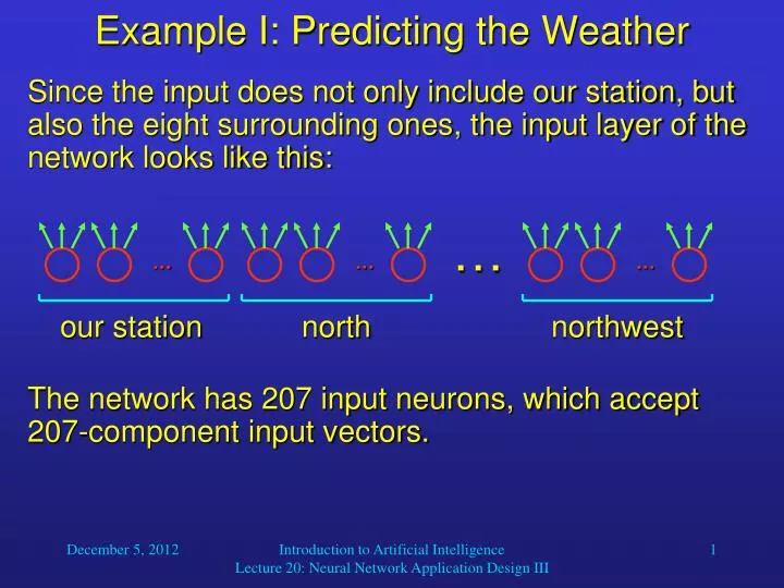
…. …. …. our station. north. northwest. Example I: Predicting the Weather. Since the input does not only include our station, but also the eight surrounding ones, the input layer of the network looks like this:. ….

E N D
… … … our station north northwest Example I: Predicting the Weather • Since the input does not only include our station, but also the eight surrounding ones, the input layer of the network looks like this: … The network has 207 input neurons, which accept 207-component input vectors. Introduction to Artificial Intelligence Lecture 20: Neural Network Application Design III
Example I: Predicting the Weather • What should the output patterns look like? • We want the network to produce a set of indicators that we can interpret as a prediction of the weather in 24 hours from now. • In analogy to the weather forecast on the evening news, we decide to demand the following four indicators: • a temperature prediction • a prediction of the chance of precipitation occurring • an indication of the expected cloud cover • a storm indicator (extreme conditions warning) Introduction to Artificial Intelligence Lecture 20: Neural Network Application Design III
Example I: Predicting the Weather • Each of these four indicators can be represented by one scaled output value: • temperature (-10… 40 degrees Celsius) • chance of precipitation (0%… 100%) • cloud cover (0… 9) • storm warning: two possibilities: • 0: no storm warning; 1: storm warning • probability of serious storm (0%… 100%) • Of course, the actual network outputs range from 0 to 1, and after their computation, if necessary, they are scaled to match the ranges specified above. Introduction to Artificial Intelligence Lecture 20: Neural Network Application Design III
Example I: Predicting the Weather • We decide (or experimentally determine) to use a hidden layer with 42 sigmoidal neurons. • In summary, our network has • 207 input neurons • 42 hidden neurons • 4 output neurons • Because of the small output vectors, 42 hidden units may suffice for this application. • Usually, more hidden units that input units are used; but as you know, no formula exists to compute the appropriate number of hidden neurons. Introduction to Artificial Intelligence Lecture 20: Neural Network Application Design III
Example I: Predicting the Weather • The next thing we need to do is collecting the training exemplars. • First we have to specify what our network is supposed to do: • In production mode, the network is fed with the current weather conditions, and its output will be interpreted as the weather forecast for tomorrow. • Therefore, in training mode, we have to present the network with exemplars that associate known past weather conditions at a time t with the conditions at t – 24 hrs. • So we have to collect a set of historical exemplars with known correct output for every input. Introduction to Artificial Intelligence Lecture 20: Neural Network Application Design III
Example I: Predicting the Weather • Obviously, if such data is unavailable, we have to start collecting them. • The amount of data that we need depends on the amount of changes in weather at our location. • For example, in Honolulu, Hawaii, we only need data for a few months, because there is little variation in the weather. • In Boston, however, we would need to cover at least one year because of dramatic changes in weather across seasons. • As we know, some winters in Boston are much harder than others, so it might be a good idea to collect data for several years. Introduction to Artificial Intelligence Lecture 20: Neural Network Application Design III
Example I: Predicting the Weather • And how about the granularity of our exemplar data, i.e., the frequency of measurement? • Using one sample per day would be a natural choice, but it would neglect rapid changes in weather. • If we use hourly instantaneous samples, however, we increase the likelihood of conflicts. • Therefore, we decide to do the following: • We will collect input data every hour, but the corresponding output pattern will be the average of the instantaneous patterns over a 12-hour period. • This way we reduce the possibility of errors while increasing the amount of training data. Introduction to Artificial Intelligence Lecture 20: Neural Network Application Design III
Example I: Predicting the Weather • Now we have to train our network. • If we use samples in one-hour intervals for one year, we have 8,760 exemplars(as a rule of thumb, though, we should ideally have about 5 to 10 times as many exemplars as there are weights in the network). • Since with a large number of samples the hold-one-out training method is very time consuming, we decide to use partial-set training instead. • The best way to do this would be to acquire a test set (control set), that is, another set of input-output pairs measured on random days and at random times. • After training the network with the 8,760 exemplars, we could then use the test set to evaluate the performance of our network. Introduction to Artificial Intelligence Lecture 20: Neural Network Application Design III
Example I: Predicting the Weather • Neural network troubleshooting: • Plot the global error as a function of the training epoch. The error should decrease after every epoch. If it oscillates, do the following tests. • Try reducing the size of the training set. If then the network converges, a conflict may exist in the exemplars. • If the network still does not converge, continue pruning the training set until it does converge. Then add exemplars back gradually, thereby detecting the ones that cause conflicts. Introduction to Artificial Intelligence Lecture 20: Neural Network Application Design III
Example I: Predicting the Weather • If this still does not work, look for saturated neurons (extreme weights) in the hidden layer. If you find those, add more hidden-layer neurons, possibly an extra 20%. • If there are no saturated units and the problems still exist, try lowering the learning parameter and training longer. • If the network converges but does not accurately learn the desired function, evaluate the coverage of the training set. • If the coverage is adequate and the network still does not learn the function precisely, you could refine the pattern representation. For example, you could include a season indicator to the input, helping the network to discriminate between similar inputs that produce very different outputs. • Then you can start predicting the weather! Introduction to Artificial Intelligence Lecture 20: Neural Network Application Design III
A Note on Setting Desired Outputs • Due to the sigmoid output function, the net input to the output units would have to be - or to generate outputs 0 or 1, respectively. • Because of the shallow slope of the sigmoid function at extreme net inputs, even approaching these values would be very slow. • To avoid this problem, it is advisable to use desired outputs and (1 - ) instead of 0 and 1, respectively. • Typical values for range between 0.01 and 0.1. • For example, for = 0.1, a desired output vector could look like this: • y = (0.1, 0.1, 0.9, 0.1) Introduction to Artificial Intelligence Lecture 20: Neural Network Application Design III
Example II: Face Recognition • Now let us assume that we want to build a network for a computer vision application. • More specifically, our network is supposed to recognize faces and face poses. • This is an example that has actually been implemented. • All information, program code, data, etc, can be found at: • http://www-2.cs.cmu.edu/afs/cs.cmu.edu/user/mitchell/ftp/faces.html Introduction to Artificial Intelligence Lecture 20: Neural Network Application Design III
Example II: Face Recognition • The goal is to classify camera images of faces of various people in various poses. • Images of 20 different people were collected, with up to 32 images per person. • The following variables were introduced: • expression (happy, sad, angry, neutral) • direction of looking (left, right, straight ahead, up) • sunglasses (yes or no) • In total, 624 grayscale images were collected, each with a resolution of 30 by 32 pixels and intensity values between 0 and 255. Introduction to Artificial Intelligence Lecture 20: Neural Network Application Design III
Example II: Face Recognition • The network presented here only has the task of determining the face pose (left, right, up, straight) shown in an input image. • It uses • 960 input units (one for each pixel in the image), • 3 hidden units • 4 output neurons (one for each pose) • Each output unit receives an additional input, which is always 1. • By varying the weight for this input, the backpropagation algorithm can adjust an offset for the net input signal. Introduction to Artificial Intelligence Lecture 20: Neural Network Application Design III
Example II: Face Recognition • The following diagram visualizes all network weights after 1 epoch and after 100 epochs. • Their values are indicated by brightness (ranging from black = -1 to white = 1). • Each 30 by 32 matrix represents the weights of one of the three hidden-layer units. • Each row of four squares represents the weights of one output neuron (three weights for the signals from the hidden units, and one for the constant signal 1). • After training, the network is able to classify 90% of new (non-trained) face images correctly. Introduction to Artificial Intelligence Lecture 20: Neural Network Application Design III
Example II: Face Recognition Introduction to Artificial Intelligence Lecture 20: Neural Network Application Design III
Example III: Character Recognition http://sund.de/netze/applets/BPN/bpn2/ochre.html Introduction to Artificial Intelligence Lecture 20: Neural Network Application Design III