Mapping and predicting the weather

1. Mapping and predicting the weather The Storm of the Century, a winter storm which struck the entire eastern half of the US on March 12, 1993.

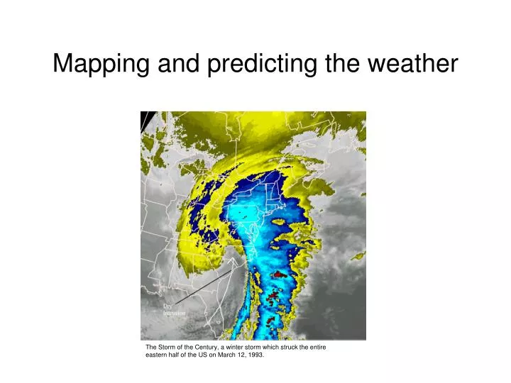
2. Mapping and predicting the weather: a history • Meteorology involves geography and cartography • Prediction is synonymous with mapping: predicting weather is best done spatially, on maps. • To arrive at where we are today with weather forecasting required innovations in how atmospheric data was collected, communicated, mapped, and analyzed.

3. Weather proverbs and folklore were the first means for predicting and understanding the weather. http://www.americanfolklore.net/folktales/rain-lore.html http://en.wikipedia.org/wiki/Weather_lore Red sky at morning, sailor take warning. Red sky at night, sailor’s delight. Visibility of stars can indicate increasing amounts of moisture in the troposphere, the lowermost layer of the atmosphere where weather takes place. This has been known to many cultures and civilizations.

4. Andean cultures used the brightness of constellations to predict the weather. Bright stars indicated more moisture in the troposphere (El Nino conditions) which could several months later lead to dry conditions (La Nina conditions). This knowledge allowed Andeans to adjust potato planting dates in anticipation of oscillating climatic conditions.

5. Weather proverbs and folklore also have a long history in the prediction and comprehension of the weather, although their accuracy can be debated. • The 189-year-old publication “The Farmers Almanac” claims 80% to 85% accuracy for the forecasts by its reclusive prognosticator, Caleb Weatherbee. • Weatherbee prepares the forecasts two years in advance using a secret formula based on sunspots, the position of the planets, and tides. • Does not meet scientific standards of weather prediction.

6. Weather logs were the first formalization of what would eventually become weather maps. Prior to late 1700's, weather data was listed in weather logs rather than spatially analyzed with maps. Integrating weather logs among places and meteorologists was thwarted by a systematic way to collect and distribute data quickly.

7. First weather maps published in 1811 by Brandes. Because it took a lot of time to assemble and plot the data, he could not predict the weather; only hindcast it. Brandes hindcasted conditions in Europe for each day of the year in 1783. He was the first to contour and plot isobars, the lines on an air pressure map. He plotted air pressure values observed across the continent and then drew in the contours by hand.

8. The invention of the telegraph aided in the rapid dissemination of weather data. Now weather observations and data could move faster from place to place. Warnings of severe weather could be communicated along telegraph wires. However, knowledge of how large weather systems travelled was poorly developed. Sketches from Morse’s notebooks showing early design of the telegraph (1840’s)

9. Development of a rapid network of telegraph stations eventually evolved to warn Atlantic cities of storms developing to the west, in the Midwest and South, shortly after 1846. Weather gauge ( instrumental) information could be telegraphed to Washington D.C. where maps were constructed. By 1860 had 45 stations reaching as far west as St. Louis

10. Signal Corps telegraph office network, (War Department, post-Civil War)

11. The network of telegraph stations increased under the US Weather Bureau administration, helped by the completion of the transcontinental railroad.

12. US Weather Bureau forecast headquarters, Washington DC, early 1900’s

13. Production and standardization of the first national weather maps in 1880’s

14. Weather Bureau transferred to Dept of Agriculture and network of local and regional forecast stations constructed. In other words, the office in Washington DC was decentralized. Telegraph was still main means of communicating weather data. However, weather over ocean was an unknown….

15. Institutional evolution of weather prediction • US Weather Bureau - US War Department (1870) • US Weather Bureau - US Department of Agriculture (1891) • US Weather Bureau - US Department of Commerce (1940) • The US Weather Bureau was renamed the National Weather Service (1970) and placed under the newly created National Ocean and Atmospheric Administration (NOAA) within the US Department of Commerce

16. Development of wireless radio technology, early 1900’s. Wireless radio communications was pioneered during WWI and used to transmit weather conditions and forecasts to and from ships at sea. Airplanes are still particularly critical today for making precise measurements of hurricane conditions and positions. View of hurricane eye from airplane.

17. But what was going on up high in the atmosphere? Initial upper atmospheric measurements initially made with kites…..note tornado in background (and the likely presence of lightning). Not a safe work environment.

18. Bi-plane with weather instruments, 1934. Planes were expensive to operate for weather data collection, and safety concerns certainly remained.

19. Balloons could be launched with people and weather instruments on board, or better, safer, and less expensive…. ..by tracking unmanned balloons, meteorologists could gain an idea of how wind speeds and directions change moving up through the troposphere.

20. Image at right shows an airplane dropping a hurricane warning notice to a crew of sponge divers of Florida. Today, airplanes drop dropsondes, which record the weather conditions in its fall to the surface. These data are transmitted back to the forecast office. Without dropsondes our knowledge and prediction of hurricane track and intensity would be greatly diminished.

21. A radiosonde is a balloon released from the surface with an attached weather recording and transmitting instrument. A dropsonde is a weather recording and transmitting instrument dropped from a plane. The instrument shown above is what records and transmits weather info on a radiosonde. It is attached underneath the balloon.

22. Radiosondes, dropsondes, and later, satellites, led to the mapping of the upper atmosphere. Shown below is the location of the polar jet stream. Colors indicate wind speed. Altitude of the polar jet stream ranges from 10-15 miles. This information could not be collected without these technological innovations.

23. Development of polar front theory(1922) , which described mid-latitude cyclones, a major weather maker. Pioneering work by Bjerknes (left) contributed to our conceptual and mathematical understanding of weather prediction. Midlatitude cyclone (left and above) encompass low pressure center and attached warm and cold fronts. Cold front is shown in blue. Warm front in red. Entire system rotates counterclockwise

24. Integration of upper-level conditions, surface conditions, and polar front theory are essential to forecasting the weather. The low pressure on the surface is a mid-latitude cyclone. Note how the winds in it are coupled to upper level flow.

25. Skew-t plot for Tallahassee Red line shows air temp and blue line shows dew point temp y-axis: tempy-axis: pressure level At what pressure level are clouds likely to form ? Invention of the skew-t plot from existing graphical methods (late 1940’s)

26. Finite difference technique of forecasting (Richardson, 1922) Grid cells used by Richardson to map his prediction of air motion determine weather patterns. Richardson’s work pioneered a method for mathematically and cartographically predicting the weather.

27. 3D block of the atmosphere showing complexity of flow To understand the finite difference technique, you have to understand some basic principles about weather prediction. At its simplest, weather prediction is predicated upon anticipating the motion of the atmosphere. Various air flow geometries of atmospheric motion are associated with certain weather conditions. Rising air is associated with cloudy conditions and low pressure. Sinking air is associated with clear conditions and high pressure. If you can predict the relative motion of the atmosphere, moving up or down, a few days in advance, you can predict the likelihood of cloudy or clear conditions. Based on these descriptions, what is the general motion of air in Montana and Idaho? (Rising). What is the general motion of air over the mid Atlantic states? (Sinking) Region of rising air: cloudy conditions and low pressure Region of sinking air: clear conditions and high pressure

28. Steps in the finite difference technique: 1. Collect data from weather stations. In this case we will collect air temperature. 2. Contour data so that temperature an be estimated for all points on the map

29. 3. Draw a grid over the entire forecast area and assign a discrete value of temperature to the center of each grid cell. The value of temperature is estimated from the contour map. 4. Repeat this same process of contouring, gridding, and assigning a value to a point at the center of each grid cell for other weather variables, like air pressure.

30. 5. Apply equations of fluid motion and thermodynamics to predict the motion of air to and from grid cells based on their temperature, air pressure, and other weather variables (dew point, wind speed and direction) These calculations will reveal general movement of air and thus the regions where there are rising (potentially cloudy) and sinking (potentially clear) atmospheric motions Richardson’s method is the basis for 3-dimensional numerical weather prediction models used today,

31. After WWII, surplus radar donated for weather forecasting

32. Early radar image of thunderstorms in Florida

33. One of the first radar images of hurricane structure, 1946

34. This was state of the art radar-based hurricane tracking in 1960

35. Now the biggest hurdle to making weather maps and forecasts was computational. The calculations were too tedious to do by hand. ENIAC-one of the first general purpose computers (1940) used to make forecasts.

36. Vacuum-tube technology (eventually replaced by transistor and integrated circuits----the “chip”) was used in ENIAC and early computers. Unreliable and prone to overheat.

37. Computer punch card---eventually replaced by magnetic tape, then floppy discs, zip discs, compact discs, and dvd’s.

38. IBM 7090 (1965) used in weather forecasting

39. The “chip” was developed in late 50’s and 60’s Refinement of integrated silicon-chip based computing, last half of 20th century.

40. Launch of first weather satellite, TIROS 1. Real time satellite tracking Launch of the first weather satellite

41. Further development of quantitative models of weather prediction • New models possible because of faster computers, better data integration and communication • Predictive model types • Global model • Nested grid model • Ensemble forecast

42. A global predictive model applies the finite difference technique over a large area, with very large grid cell sizes. This allows meteorologists to predict the weather by looking “upstream” to see what kinds of conditions are coming their way. Remember, weather systems tend to flow from west to east. One of the weaknesses of this model is that it cannot make local weather predictions: the grid cells are too large. It is also very computationally intensive.

43. A 24-hour global forecast system (GFS) prediction of potential precipitation. The map shows the predicted weather for 8 pm Thursday night Eastern Standard Time (which is midnight, or 0Z Friday on the Prime Meridian). I downloaded this map Thursday morning, March 13th. As this is a 24 hour prediction, the model was run Wednesday night, 8 pm Eastern Standard Time. (Also see this link: http://www.wunderground.com/modelmaps/maps.asp?model=GFS&domain=TA)

44. A nested grid predictive model also uses the finite difference technique, but it combines the large scale global grid with a smaller grid with much finer grid cells. This allows forecasters to see and predict the big picture, while also accounting for local conditions. The smaller grid cells in the nested grid allow more detail for local forecasts.

45. A 24-hour nested grid predictive model (NGM) showing areas of potential precipitation. This is the prediction for 8 am Friday Eastern Standard Time (which is noon, or 12Z Thursday on the Prime Meridian). I downloaded this map Thursday morning, March 13th. As this is a 24 hour prediction, the model was run Thursday morning 8 am Eastern Standard Time.

46. Hurricane forecasters look at the way models agree and disagree with each other. Each of the lines below is predicted track from different computer models (NGM and GFS models are two of them). By looking at how the models agree and disagree a measure of how much certainty in the track can be estimated. If models disagree to a large extent, there is a greater sensitivity to local conditions . Small differences in initial conditions input into the models can lead to vastly different forecasts The result is a much harder to predict hurricane.

47. Which hurricane is more sensitive to the local conditions surrounding it? In other words, which storm, when weather variables are fed into the forecast models, is more dependent upon small differences in them? The white envelope indicates the potential 1-3 day area in which the eye of the hurricane may pass. (The atmospheric and oceanic conditions with Ivan (left) are much more difficult to predict based on the shape of the white cone. Very localized variations in air temperature, ocean temperature, or winds around the storm could cause Ivan to shift tracks over a very wide area. With Noel, any local variability in air and ocean temperatures or winds are unlikely to have any effect on the outcome of the storm track. You could enter a range of initial conditions in the models for Noel (right) and the models would likely agree with each other.

48. Predicting hurricane intensity is more difficult than predicting its track. This is because the conditions that determine intensity exist on much smaller scales and are difficulty to measure within and around the hurricane. These parameters are a challenge to integrate into track forecast models.

49. Hurricane Charley, 2004 The detection of “hot tower” thunderstorms in hurricanes are thought to herald an increase in strengthening (an example of remote sensing)

50. NEXRAD Doppler radar coverage for the US, another geographic-meteorologic innovation