Download
1 / 33
330 likes | 475 Views
Stellar PHOTOMETRY ON TIMESCALES OF TENTHS OF SECONDS TO YEARS. Jeff Wilkerson Luther College MSU Mankato October 11, 2007. Our Observations Science Goals Data Acquisition and Analysis Photometric Limits Variable Star Observations. What We Do.

E N D
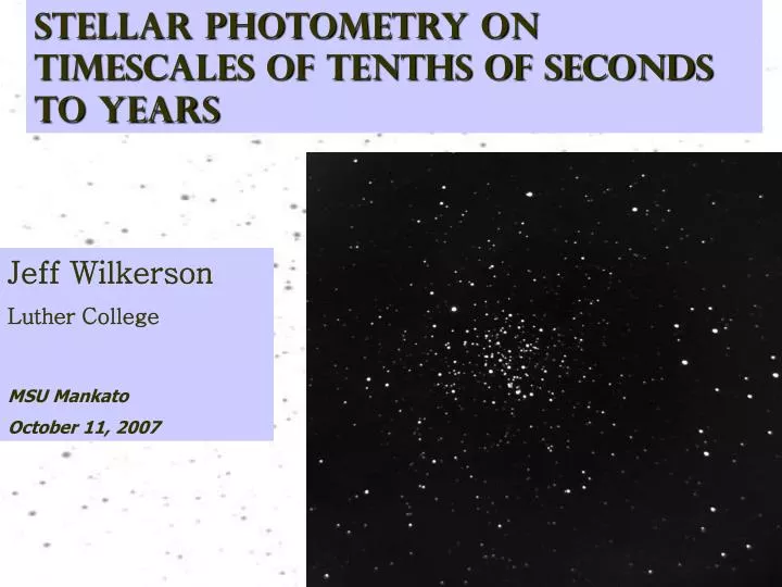
Stellar PHOTOMETRY ON TIMESCALES OF TENTHS OF SECONDS TO YEARS Jeff Wilkerson Luther College MSU Mankato October 11, 2007
Our Observations • Science Goals • Data Acquisition and Analysis • Photometric Limits • Variable Star Observations
What We Do We image 3 clusters per year: M23 and two others Image durations: 2 to 12 seconds, unfiltered Campaign durations: 5 to 7 months Return to a cluster at least once BVRI photometry at least once for color correction to magnitude conversion and knowledge of variable star colors Result: tens of thousands of images per cluster per year Equipment: 12” Meade Schmidt-Cassegrain; Apogee AP6E camera How did we get here? What are our goals?
All images acquired with a 12” Meade LX200 and Apogee AP6E camera
Student Participation: Zebadiah Howes Buena Vista Univ. Travis DeJong Dordt College Forrest Bishop Decorah High School Ujjwal Joshi Nathan Rengstorf Andrea Schiefelbein Todd Brown Brajesh Lacoul Kari Frank Alex Nugent Robyn Siedschlag Siri Thompson Matt Fitzgerald Heather Lehmann Amalia Anderson Hilary Teslow Support: Roy J. Carver Charitable Trust (Grant #00-50) Luther College R.J. McElroy Trust/Iowa College Foundation
Our Observational Goals: • I. Brief changes in apparent stellar flux • Occultation and microlensing events • Flare stars • II. Very long timescale changes in stellar luminosity • Luminosity stability • Solar-like cycles6 • Low-amplitude, ultra-long period pulsation • III. Traditional Stellar Variability • Surveys of new variable stars • Locate detached and semi-detached eclipsing binaries in clusters1 • Locate contact eclipsing binaries in clusters2 • Period/amplitude variations in contact systems3 • Period-to-period variability in long period variables • Search for cataclysmic variables in clusters4 • Search for transiting planets5 • Rotating variable star periods in young clusters7 • Wyithe, J.S.B, and Wilson, R.E. 2002, ApJ, 571, 293 • Rucinski, S.M. 1998, AJ, 116, 2998 • Paczynski, B., et al. 2006, MNRAS, 368, 1311 • Mochejska, B.J., et al. 2004, AJ, 128, 312 • Mochejska, B.J., and Stanek, K.Z. 2006, AJ, 131,1090 • Lockwood G.W., et al. 1997 ApJ, 485, 780-811 • Herbst W. and Mundt R., 2005, ApJ, 633, 967-985
Dense Object 60 50 40 30 Negative 5.4 sigma fluctuation 20 10 0 2800 3000 3200 3400 3600 3800 4000 4200 Signal (ADU)
Estimate the number of occultation events per image: Depends on # of objects in the field and the likelihood of any object hitting a star tmin depends on image duration and photometric precision. If a star is occulted for 10% of the image duration And s/m=2.5% then a 4s event results. Assume a power law distribution of occulting objects: Event rate at any threshold goes as vx+2 and (tmin)x+1 e.g., if x = -4 (as for known KBOs) event rate goes as v-2 and (tmin)-3; a similar analysis for microlensing events yields an event rate proportional to v-2/3.
HR DIAGRAM WITH INSTABILITY STRIPS From “Understanding Variable Stars” by Percy (Cambridge, 2007)
DATA PROCESSING • CALIBRATION • Dark Noise Correction • Flat Fielding • ALIGNMENT • Use a single frame for entire data set • STAR ID & EXTRACTION • Aperture photometry for signal determination • 256 Background regions • INTRA-NIGHT NORMALIZATION • INTER-NIGHT NORMALIZATION • MAGNITUDE CONVERSION All Analysis done with code developed in IDL
Frame Normalization • Identify four reference images from throughout the night • Calculate average flux for each star in all four frames – this is the reference signal • Determine the signal of each star in the frame to be normalized – this is the sample signal • Calculate (ref. signal/sample signal) for each star • Normalization factor = median of all ratios in (4)
INTRA-NIGHT NORMALIZATION FACTORS Stars appear dimmer lower in the sky due to increased atmospheric scattering.
Stellar color is important in atmospheric scattering Use Web Version of the BDAcatalog for colors (Mermilliod and Paunzen , http://www.univie.ac.at/webda//).
How is our photometry? Define Short-term Photometric Resolution (STPR) as s/m for a Gaussian fit to a histogram of several hundred signal measurements for a given star. At large signal values STPR approaches a constant (plateau) value determined by our frame normalization, itself limited by scintillation. For faint stars STPR increases as signal-1. In between STPR increases as signal-1/2. Counting statistics of the stellar signal measurement dominate STPR in this region. Functional fits shown of form: STPR=[(C1)² + (C2signal-1/2)² + (C3signal)2]1/2
Photometric resolution is determined largely by atmospheric scintillation and improves with the altitude of the observation.
We define long-term photometric resolution (LTPR) as s/m for the nightly average signal measure of a given star over an entire campaign
On each night we look at a set of several hundred brighter stars with suspected variables remove. We measure the scatter of the nightly mean divided by the campaign mean. In this way we identify nights of unacceptable photometric quality.
Use Web Version of the BDAcatalog for magnitudes (Mermilliod and Paunzen , http://www.univie.ac.at/webda//). Find an empirical color equation for the system and apply it.
Observation of Variable Stars in the M23 Field To date we have identified 36 variables in the M23 field. Of these, one appears in the GCVS (http://www.sai.msu.su/groups/cluster/gcvs/gcvs/) as a semi-regular variable and one more appears as an eclipsing binary in the ASAS catalog (http://archive.princeton.edu/~asas/). The remainder appear to be newly discovered variables. Of the variable stars observed we tentatively classify 4 of them as “long period” (P>1 day) eclipsing binaries, 3 as “short period” eclipsing binaries and the remainder as long period pulsating stars.
COLOR/MAGNITUDE DIAGRAMS The left diagram is constructed for the brightest stars in the field, including main sequence cluster members. The middle diagram includes the middle 480 stars, ranked in intensity. The right diagram includes only the faintest stars in the field. As expected, the long period pulsating stars are among the reddest in the field. The eclipsing binaries lie near the M23 main sequence. BVRI color measurements were made utilizing a nearby low-precision standard field from the Loneos Catalogue. (Henden, A., ftp://ftp.nofs.navy.mil/pub/outgoing/aah/photom/ubvri.cat)
Short Period Eclipsing Binaries Period = 0.32866 days Period = 0.54550 days Period = 0.20730 days
Search for Period Changes in Short Period Eclipsing Binaries
Sample Light Curves of Long Period Variables Star 317 Star 414 Star 850 Star 338
Sample Light Curves of Long Period Variables Star 981 Star 1223 Star 294 Star 1654
Other Interesting Stars Long-term “drift” star candidate Short-period pulsating variable
CONCLUSION • We survey three open cluster regions per year, collecting 50,000 or more images of each field over a ~six month time span. • Can detect variability on timescales of minutes to years with a precision of a few percent or better • By summing images can survey stars from 8th to 19th magnitude. • Have found many new variable stars in field of open cluster M23; these provide a rich set of objects for long-term study • Have completed a second campaign on NGC2286; so many more clusters to look at.