Download
1 / 7
80 likes | 163 Views
Potential Step Methods – From Chronoamperometry to Double-potential Step Chronocoulometry. Okay, what if we step out to rising wave region?. i c. i l. -. E vs. Ref. +. i a. Case IB: Concs of O and R must obey Nernst Equation.

E N D
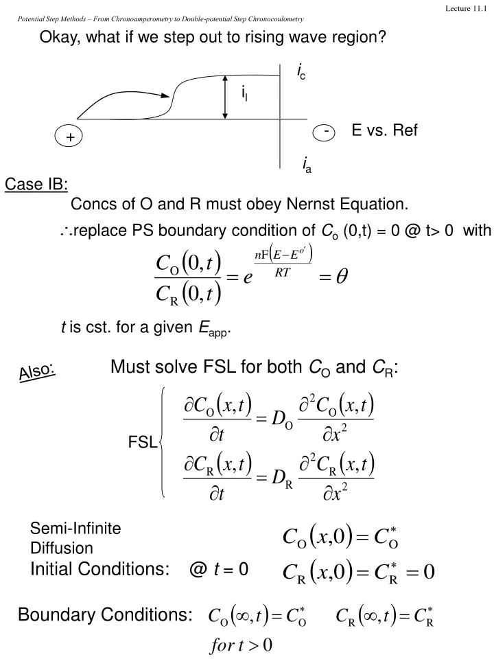
Potential Step Methods – From Chronoamperometry to Double-potential Step Chronocoulometry Okay, what if we step out to rising wave region? ic il - E vs. Ref + ia Case IB: Concs of O and R must obey Nernst Equation. replace PS boundary condition of Co (0,t) = 0 @ t> 0 with t is cst. for a given Eapp. Must solve FSL for both CO and CR: Also: FSL Semi-Infinite Diffusion Initial Conditions: @ t = 0 Boundary Conditions:
Potential Step Methods – From Chronoamperometry to Double-potential Step Chronocoulometry Solving: From FFL: Cottrell Equation for ANY Efinal At sufficiently -Eapp (Ef), q 0 and we get equation for Case IA, id(t)!! Knowing erfc(0) = 1, we get
Potential Step Methods – From Chronoamperometry to Double-potential Step Chronocoulometry t1 t values it(E) t2 t1 < t2 E vs. Ref Okay, now we consider Case IIA, but assume Quasi – Reversible Behavior: Reversible: Quasi – Rev: in between Totally Irrev: Solving: Butler – Volmer (E-T) Includes Mass – Transfer (But E-T is there too) i(t) = [i in absence of MT limitations]*f(H,t) Accounts for MT Effects
Potential Step Methods – From Chronoamperometry to Double-potential Step Chronocoulometry For small values, Linearized Form Both O/R present Step of Einit (Eeq) to Efinal gives h. Plot of i vs t1/2 has i without MT effects at intercept. This is the instantaneous current, iinst., (w/o MT) and is only due to kinetic limitations. Obtaining the iinst. as function of h and plotting gives io; Recall B-V at small h : (at - overpotential) iinst.
Potential Step Methods – From Chronoamperometry to Double-potential Step Chronocoulometry Summarizing: 1. Both O/R present 2. 3. step to small (away from Eeq) 4. look at i(t) at short times as function of ; 5. plot i(t) vs t1/2, at a given , get iinst from intercept 6. plot iinst vs. , get io from slope. 7. get from What if we have only O? but due to fact so, Get from vs. Intercept (t = 0)
Potential Step Methods – From Chronoamperometry to Double-potential Step Chronocoulometry Summarizing: 1. Only O present 2. 3. step to small h (“foot” of wave) 4. plot i vs. t1/2 , extrapolate to t = 0 , get intercept, Okay, now we consider Case IIA, but assume Totally Irreversible Behavior:
Potential Step Methods – From Chronoamperometry to Double-potential Step Chronocoulometry id 1.0 0 -2 -1 0 +1 So, wave shape of any irreversible couple is above. Also, we see that at sufficient h, the Reversible O R reaction i small large 0 0 t So if we “push” on ET rxn, make rev. look irrev. Wait irrev becomes rev.