Download
1 / 31
320 likes | 425 Views
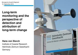
Concepts of Detection and Attribution. Hans von Storch Institute for Coastal Research GKSS Research Center, Geesthacht, Germany and Meteorological Institute, Hamburg University. Person: Hans von Storch. Hans von Storch director of Institute for Coastal Research @ GKSS

E N D
Concepts of Detection and Attribution Hans von Storch Institute for Coastal ResearchGKSS Research Center, Geesthacht, Germanyand Meteorological Institute, Hamburg University
Person: Hans von Storch • Hans von Storch • director of Institute for Coastal Research @ GKSS • professor for Meteorology at the Meteorological Institute @ U Hamburg • author of „Statistical Analysis in Climate Research“ @ Cambridge U Press (with Francis Zwiers) and other books. • doctor h.c. at Natural Science Faculty @ U Göteborg
Detection and attribution of ongoing change Omstedt, 2005
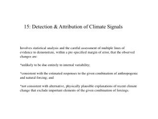
The question if we „see something“ supporting the reality of a human influence on climate – needs the adoption of a mathematical language. Determination of man-made climate change is not a matter of theory, but of assessing data. The framework is of statistical nature, and the results are probability statements condition upon certain assumptions. The whole process is called „detection and attribution“.
„Significant“ trends • Often, an anthropogenic influence is assumed to be in operation when trends are found to be „significant“. • If the null-hypothesis is correctly rejected, then the conclusion to be drawn is – if the data collection exercise would be repeated, then we may expect to see again a similar trend. • Example: N European warming trend “April to July” as part of the seasonal cycle. • It does not imply that the trend will continue into the future (beyond the time scale of serial correlation). • Example: Usually September is cooler than July.
„Significant“ trends Establishing the statistical significance of a trend is a necessary condition for claiming that the trend would represent evidence of anthropogenic influence. Claims of a continuing trend require that the dynamical cause for the present trend is identified, and that the driver causing the trend itself is continuing to operate. Thus, claims for extension of present trends into the future require- empirical evidence for an ongoing trend, and- theoretical reasoning for driver-response dynamics, and- forecasts of future driver behavior.
Detection and attribution of non-natural ongoing change • Detection of the presence of non-natural signals: rejection of null hypothesis that recent trends are drawn from the distribution of trends given by the historical record. Statistical proof. • Attribution of cause(s): Non-rejection of the null hypothesis that the observed change is made up of a sum of given signals. Plausibility argument. • History: • Hasselmann, K., 1979: On the signal-to-noise problem in atmospheric response studies. Meteorology over the tropical oceans (B.D.Shaw ed.), pp 251-259, Royal Met. Soc., Bracknell, Berkshire, England. Hasselmann, K., 1993: Optimal fingerprints for the detection of time dependent climate change. J. Climate 6, 1957 - 1971 Hasselmann, K., 1998: Conventional and Bayesian approach to climate change detection and attribution. Quart. J. R. Meteor. Soc. 124: 2541-2565
Simulation data: internally generated by a very large number of chaotic processes. Dynamical “cause” for real world’s natural unforced variability best explained as in models. Where does the stochasticity come from? Stochasticity is a mathematical construct to allow an efficient description of the (simulated and observed) climate variability.
With the help of the limited empirical evidence from instrumental observations, possibly after suitable extraction of the suspected „non-natural“ signal. By accessing long „control runs“ done with quasi-realistic climate models. By projection of the signal on a proxy data space, and by determining the statistics of the latter from geoscience indirect evidence (e.g., tree rings). How do we determine the „natural climate variability“?
Cases of Global Climate Change Detection Studies In the 1990s … weak, not well documented signals. Example: Near-globally distributed air temperature IDAG (2005), Hegerl et al. (1996), Zwiers (1999) In the 2000s … strong, well documented signals Examples: Rybski et al. (2006) Zorita et al. (2009) IDAG, 2005: Detecting and attributing external influences on the climate system. A review of recent advances. J. Climate 18, 1291-1314 Hegerl, G.C., H. von Storch, K. Hasselmann, B.D. Santer, U. Cubasch, P.D. Jones, 1996: Detecting anthropogenic climate change with an optimal fingerprint method. J. Climate 9, 2281-2306 Zwiers, F.W., 1999: The detection of climate change. In: H. von Storch and G. Flöser (Eds.): Anthropogenic Climate Change. Springer Verlag, 163-209, ISBN 3-540-65033-4 Rybski, D., A. Bunde, S. Havlin,and H. von Storch, 2006: Long-term persistence in climate and the detection problem. Geophys. Res. Lett. 33, L06718, doi:10.1029/2005GL025591 Zorita, E., T. Stocker and H. von Storch: How unusual is the recent series of warm years? Geophys. Res. Lett.
Trend in air temperature 1965-1994 Signal or noise? 1916-1945 Hegerl et al., 1996
“Guess patterns” The reduction of degrees of freedom is done by projecting the full signal S on one or a few several “guess patterns” Gk, which are assumed to describe the effect of a given driver. S = k k Gk + n with n = undescribed part. Example: guess pattern supposedly representative of increased CO2 levels Hegerl et al., 1996
Trends in a scenario calculation until 2100 Trends in temperature until 1995 Hegerl et al., 1996
Attribution diagram for observed 50-year trends in JJA mean temperature. Zwiers, F.W., 1999: The detection of climate change. In: H. von Storch and G. Flöser (Eds.): Anthropogenic Climate Change. Springer Verlag, 163-209, ISBN 3-540-65033-4 The ellipsoids enclose non-rejection regions for testing the null hypothesis that the 2-dimensional vector of signal amplitudes estimated from observations has the same distribution as the corresponding signal amplitudes estimated from the simulated 1946-95 trends in the greenhouse gas, greenhouse gas plus aerosol and solar forcing experiments.
attribution From: Hadley Center, IPCC TAR, 2001
Global mean air temperature Statistics of ΔTL,m, which is the difference of two m-year temperature means separated by L years. Temperature variations are modelled as Gaussian long-memory process, fitted to various reconstructions of historical temperature (Moberg, Mann, McIntyre) The Rybski et al- approach Historical Reconstructions – their significance for “detection”
Historical Reconstructions – their significance for “detection” Temporal development of Ti(m,L) = Ti(m) – Ti-L(m) divided by the standard deviation of the m-year mean reconstructed temp record for m=5 and L=20 (top), andfor m=30 and L=100 years. The thresholds R = 2, 2.5 and 3σ are given as dashed lines. Rybski et al., 2006
Counting extremely warm years • Among the last 17 years, 1990-2006, there were the 13 warmest years since 1880 (i.e., in 127 samples) – how probable is such an event if the time series were stationary? • Monte-Carlo simulations taking into account serial correlation, either AR(1) (with lag-1 correlation ) or long-term memory process (with Hurst parameter H=0.5+d). • Best guesses • 0.8 d 0.3 (very uncertain) Zorita, et al 2009
Regional: the Baltic Sea catchment Bhend, J., and H. von Storch, 2007: Consistency of observed winter precipitation trends in northern Europe with regional climate change projections, Climate Dynamics, DOI 10.1007/s00382-007-0335-9 Bhend, J., and H. von Storch, 2009: Consistency of observed temperature trends in the Baltic Sea catchment area with anthropogenic climate change scenarios, Boreal Environment Research, accepted
Detection: “Is the observed change different from what we expect due to internal variability alone?” – not doable at this time, since natural variability not known well enough. Trends – are there significant trends? – no useful results. Consistency: “Are the observed changes similar to what we expect from anthropogenic forcing?”Doable: Plausibility argument using an a priori known forcing. Options
Consistency analysis: attribution without detection The check of consistency of recent and ongoing trends with predictions from dynamical (or other) models represents a kind of „attribution without detection“. The idea is to estimate the driver-related change from a (series of) model scenarios (or predictions), and to compare this “expected change” with the recent trend. If recent change expectation, then we may conclude that the recent change is not due to the suspected driver, at least not completely.
DJF mean precipitation in the Baltic Sea catchment Example: Recent 30-year trend Trend of DJF precip according to different data sources.
Consistency analysis • Expected signals • Six simulations with regional coupled atmosphere-Baltic Sea regional climate model RCAO (Rossby-Center, Sweden) • three simulations forced with HadCM3 global scenarios, three with ECHAM4 global scenarios; 2071-2100 • two simulation exposed to A2 emission scenario, two simulations exposed to B2 scenario; 2071-2100 • two simulations with present day GHG-levels; 1961-90 • Regional climate change in the four scenarios relatively similar.
Regional DJF precipitation Δ=0.05%
Consistency analysis: Baltic Sea catchment • Consistency of the patterns of model “predictions” and recent trends is found in most seasons. • A major exception is precipitation in JJA and SON. • The observed trends in precipitation are stronger than the anthropogenic signal suggested by the models. • Possible causes:- scenarios inappropriate (false)- drivers other than CO2 at work (industrial aerosols?)- natural variability much larger than signal (signal-to-noise ratio 0.2-0.5).
Overall summary • How do we know that human influence is changing (regional) climate? • Statistical analysis of ongoing change with distribution of “naturally” occurring changes – detection, statistical proof.- ok for global and continental scale temperature. • In the 1990s, advanced statistical analysis needed, today also done with simpler methodology. • Consistency of continental temperature change with projected (expected) change in regions such as Baltic Sea catchment (temperature and related variables); problem with precipitation.
Thanks for your attention When you want more to know: http://coast.gkss.de/staff/storch Contact: hvonstorch@web.de