Download
1 / 31
370 likes | 559 Views
The concepts of Detection and Attribution. Hans von Storch Institute for Coastal Research GKSS Research Center, Geesthacht, Germany and Meteorological Institute, Hamburg University.

E N D
The concepts of Detection and Attribution Hans von Storch Institute for Coastal ResearchGKSS Research Center, Geesthacht, Germanyand Meteorological Institute, Hamburg University Global Warming - Scientific Controversies in Climate Variability International seminar meeting at The Royal Institute of Technology (KTH), Stockholm, Sweden, September 11-12th 2006
Detection and attribution • Detection means – finding in a record of observations evidence for a contamination of the „natural variability“ by man-made signals. A statistical problem. • Attribution means – finding the most plausible explanation for the cause of the detected contamination. A plausibility argument. Concept introduced by Klaus Hasselmann, first in 1979, and later in a framework geared towards the problem of anthropogenic climate change in 1993. Hasselmann, K., 1979: On the signal-to-noise problem in atmospheric response studies. Meteorology over the tropical oceans (B.D.Shaw ed.), pp 251-259, Royal Met. Soc., Bracknell, Berkshire, England. Hasselmann, K., 1993: Optimal fingerprints for the detection of time dependent climate change. J. Climate 6, 1957 - 1971
The detection problem: Test of the nullhypothesis: „considered climate signal is consistent with natural climate variability“ with Strepresenting the signal to be examined, whether it is consistent with natural climate variability or not, and describing the distibution of the present climate with parameters and . Problem is to determineStand its distribution P.
The attribution problem After we have found a signal to lie outside the range of natural variations, the question arises whether this signal can be causally related to an external factor. Usually, there are many factors, but climatological theory reduces the candidates to just a few (e.g., greenhouse gases, volcanic aerosols, solar effects). Then, that mix of processes is attributed to the signal, which fits best to the a-priori assumed link between cause and effect. This may take the form of a best-fit or as the result of a non-rejection of a null hypothesis. Detection is a strictly statistical problem. Attribution is based on a plausibility argument.
The attribution problem If the theory / knowledge claims provide numerically accurate “responses”, then also the coefficients γk are „known“. Then instead of a best-fit approach, a test using the hypothesis H0: γk = expected value can be formulated – and attribution is considerd to be achieved when H0 is NOT rejected.
Where does the stochasticity come from? • Observational data: irregular spatial coverage, observational errors, limited observation time span. And natural unforced variability. • Simulation data: internally generated by a very large number of chaotic processes.Stochasticity as mathematical construct to allow an efficient description of the simulated (and observed) climate variability. • Dynamical “cause” for natural unforced variability as in models.
Institut für Küstenforschung I f K Noise or deterministic chaos? Mathematical construct of randomness – an adequate concept for description of features resulting from the presence of many chaotic processes.
Noise as nuisance: masking the signal The 300 hPa geopotential height fields in the Northern Hemisphere: the mean 1967-81 January field, the January 1971 field, which is closer to the mean field than most others, and the January 1981 field, which deviates significantly from the mean field. Units: 10 m
How do we determine the control climate ? • With the help of the limited empirical evidence from instrumental observations, possibly after suitable extraction of the suspected „non-natural“ signal. • By projection of the signal on a proxy data space, and by determining the stats of the latter from geoscience indirect evidence (e.g., tree rings). • By accessing long „control runs“ done with quasi-realistic climate models
Signal or noise? Trend in air temperature 1965-1994 1916-1945
Formulation the null hypothesis • Reduction of dimension be projection of the full fields on „guess pattern(s)“ Gk. • Guess patterns represent our expectations about the anthropogenic signals. (They may be false, but the test is still correct, but with little power.) • Guess patterns may originate from numerical experiments on the suspected mechanisms, or from other reasoning (paleoclimatic/historical analogues; theoretical considerations). • Test whether αk consistent with natural variability.
Expected anthropogenic GHG signal • … emerges most clearly in the last decades • … accelerates with time • … manifests itself in a strong increase of temperature, not with an unprecedented level of temperature. • The detection variable is “change of T”, not “state of T”.
From: Hadley Center, IPCC TAR, 2001 attribution
Detection – does it depend on the hockeystick? Rybski, D., A. Bunde, S. Havlin,and H. von Storch, 2006: Long-term persistence in climate and the detection problem. Geophys. Res. Lett. 33, L06718, doi:10.1029/2005GL025591
Historical Reconstructions – their significance for “detection” • Statistics of ΔTL,m, which is the difference of two m-year temperature means separated by L years. • Temperature variations are modelled as Gaussian long-memory process, fitted to the various reconstructions.
Historical Reconstructions – their significance for “detection” Temporal development of Ti(m,L) = Ti(m) – Ti-L(m) divided by the standard deviation (m,L) of the considered reconstructed temp record for m=5 and L=20 (top), andfor m=30 and L=100 years. The thresholds R = 2, 2.5 and 3 are given as dashed lines.
Conclusions • Detection of anomalous conditions and attribution to specific causes is a well defined and developed concept in climate change studies. • Detection is a strictly statistical problem; attribution is a plausibility argument. • A-priori guidance by quasi-realistic models most helpful if not mandatory. • Improvement of data base for estimating variability with the help of quasi-realistic models most helpful if not mandatory. • Ongoing climate variations can not be explained by natural climate variations alone. Detection has succeeded. • A significant proportion of the detected signal can be attributed to increased levels of carbon dioxide. • All available historical reconstructions, from MBH to Moberg, lead to a very small risk of rejecting the null hypothesis of only natural variablity. Detection is independent of the hockey-stick claim.
Institut für Küstenforschung I f K Noise as a constitutive element Numerical experiment with ocean model: standard simulation with steady forcing (wind, heat and fresh water fluxes) plus random zero-mean precipitation overlaid. forcing Mikolajewicz, U. and E. Maier-Reimer, 1990 Example for Stochastic Climate Model at work. response
Noise as constitutive element = (T) Idealized energy balance
Institut für Küstenforschung I f K Integration of a zero–dimensional energy balance model with constant transmissivity and temperature dependent albedo no noise evolution from different initial values with noise evolution with slightly randomized transmissivity
Example of a local detection study. Pfizenmayer (2002) Estimated wave energy impinging on the West Coast of Jutland (Sylt),derived with a downscaling model from large scale monthly mean atmospheric states in operational analyses („reconstruction“), in a control simulation (T42 control) and in a climate change simulation (T42 transient).The energy increases even though the storm activity does hardly so.
References Zwiers, F.W., 1999: The detection of climate change. In: H. von Storch and G. Flöser (Eds.): Anthropogenic Climate Change. Springer Verlag, 163-209, ISBN 3-540-65033-4 vonStorch, H., J.-S. von Storch, and P. Müller, 2001: Noise in the Climate System – ubiquituos, constitutive and concealing. In B. Engquist and W. Schmid (eds.) Mathematics Unlimited – 2001 and beyond. Part II. Springer Verlag, 1179-1194 Hegerl, G.C. , K.H. Hasselmann, U. Cubasch, J.F.B. Mitchell, E. Roeckner, R. Voss and J. Waszkewitz, 1997: Multi-fingerprint detection and attribution analysis of greenhouse gas, greenhouse gas-plus-aerosol and solar forced climate change. Clim. Dyn. 13, 613-634 Pfizenmayer and H. von Storch, 2001: Anthropogenic climate change shown by local wave conditions in the North Sea. Climate Res. 19, 15-23 Rybski, D., A. Bunde, S. Havlin,and H. von Storch, 2006: Long-term persistence in climate and the detection problem. Geophys. Res. Lett. 33, L06718, doi:10.1029/2005GL025591
Specific problem in climate applications: usually very many (>103) degrees of freedom, but the signal of change resides on in a few of these degrees of freedom. Example: Signal = (2, 0, 0, ...0)with all componentsindependent. Power of detecting thesignal, if different degrees of freedom are considered. Thus, the dimension of the problem must be reduced before doing anything further. Usually, only very few components are selected, such as 1 or 2.
2-patterns problem (Hegerl et al. 1997) • guess patterns for climate change mechanisms taken as first EOFs of a climate change simulation on that mechanism. • only CO2 increase • increase of CO2 and industrial aerosols as well. • orthogonalisation of the two patterns • estimation of natural variability through GCM control simulations done at MPI in Hamburg, GFDL in Princeton and HC in Bracknell.
30 year trends detection
50 year trends attribution