Download

1 / 49
500 likes | 527 Views
Dimension Reduction - PCA. P rinciple C omponent A nalysis. The Goals. Reduce the number of dimensions of a data set. Capture the maximum information present in the initial data set. Minimize the error between the original data set and the reduced dimensional data set.

E N D
Dimension Reduction - PCA Principle Component Analysis סמינריון במתמטיקה ביולוגית
The Goals • Reduce the number of dimensions of a data set. • Capture the maximum information present in the initial data set. • Minimize the error between the original data set and the reduced dimensional data set. • Simpler visualization of complex data. סמינריון במתמטיקה ביולוגית
The Algorithm • Step 1: Calculate the Covariance Matrix of the observation matrix. • Step 2: Calculate the eigenvalues and the corresponding eigenvectors. • Step 3: Sort eigenvectors by the magnitude of their eigenvalues. • Step 4: Project the data points on those vectors. סמינריון במתמטיקה ביולוגית
The Algorithm • Step 1:Calculate the Covariance Matrix of the observation matrix. • Step 2: Calculate the eigenvalues and the corresponding eigenvectors. • Step 3: Sort eigenvectors by the magnitude of their eigenvalues. • Step 4: Project the data points on those vectors. סמינריון במתמטיקה ביולוגית
PCA – Step 1: Covariance Matrix C • - Data Matrix סמינריון במתמטיקה ביולוגית
Covariance Matrix - Example סמינריון במתמטיקה ביולוגית
The Algorithm • Step 1: Calculate the Covariance Matrix of the observation matrix. • Step 2: Calculate the eigenvalues and the corresponding eigenvectors. • Step 3: Sort eigenvectors by the magnitude of their eigenvalues. • Step 4: Project the data points on those vectors. סמינריון במתמטיקה ביולוגית
Example Linear Algebra Review – Eigenvalue and Eigenvector • C - a square nn matrix eigenvalue eigenvector סמינריון במתמטיקה ביולוגית
Singular Value Decomposition סמינריון במתמטיקה ביולוגית
SVD Example Let us find SVD for the matrix • First, compute XTX: • Second, find the eigenvalues of XTX and the corresponding eigenvectors: ( use the following formula - ) סמינריון במתמטיקה ביולוגית
SVD Example - Continue • Now, we obtain the U and Σ : • And the decomposition C=UΣVT: סמינריון במתמטיקה ביולוגית
The Algorithm • Step 1: Calculate the Covariance Matrix of the observation matrix. • Step 2: Calculate the eigenvalues and the corresponding eigenvectors. • Step 3: Sort eigenvectors by the magnitude of their eigenvalues. • Step 4: Project the data points on those vectors. סמינריון במתמטיקה ביולוגית
PCA – Step 3 • Sort eigenvectors by the magnitude of their eigenvalues סמינריון במתמטיקה ביולוגית
The Algorithm • Step 1: Calculate the Covariance Matrix of the observation matrix. • Step 2: Calculate the eigenvalues and the corresponding eigenvectors. • Step 3: Sort eigenvectors by the magnitude of their eigenvalues. • Step 4: Project the data points on those vectors. סמינריון במתמטיקה ביולוגית
Project the input data onto the principal components. The new data values are generated for each observation, which are a linear combination as follows: PCA – Step 4 • score • observation • principal component • loading (-1 to 1) • variable סמינריון במתמטיקה ביולוגית
X3 1st PC Projections Var(PC2) Var(PC1) X2 2nd PC X1 PCA - Fundamentals • The first PC is the eigenvector with the greatest eigenvalue for the covariance matrix of the dataset. • The Eigenvalues are also the variances of the observations in each of the new coordinate axes סמינריון במתמטיקה ביולוגית
x2 1st PC x3 2nd PC x1 PCA: Scores Obs. i • The scores are the places along the component lines where the observations are projected. סמינריון במתמטיקה ביולוגית
PCA: Loadings x2 x2 1st PC a3 a2 x3 Cos(a)=X/PC a1 x1 x3 x1 • The loadings bpc,k (dimension a, variable k) indicate the importance • of the variable k to the given dimension. • bpc,k is the direction cosine (cos a) of the given component line vs. the xk coordinate axis. סמינריון במתמטיקה ביולוגית
PCA - Summary • Multivariate projection technique. • Reduce dimensionality of data by transformingcorrelated variables into a smaller number of uncorrelated components. • Graphical overview. • Plot data in K-Dimensional space. • Directions of maximum variation. • Best preserves the variance as measured in the high-dimensional input space. • Projection of data onto lower dimensional planes. סמינריון במתמטיקה ביולוגית
Biological Background סמינריון במתמטיקה ביולוגית
c Reverse Transcriptase סמינריון במתמטיקה ביולוגית
Areas Being Studied With Microarrays • To compare the expression of a protein (gene) between two or more tissues. • To check whether a protein appears in a specific tissue. • To find the difference in gene expression between a normal and a cancerous tissue. סמינריון במתמטיקה ביולוגית
cDNA Microarray Experiments • Different tissues, same organism (brain v. liver). • Same tissue, different organisms. • Same tissue, same organism (tumour v. non-tumour). • Time course experiments. סמינריון במתמטיקה ביולוגית
Microarray Technology • Method for measuring levels of expression of thousands of genes simultaneously. • There are two types of arrays: • cDNA and long oligonucleotide arrays. • Short oligonucleotide arrays. • Each probe is ~25 nucleotide long. • 16-20 probes for each gene. סמינריון במתמטיקה ביולוגית
Probe: oligos/cDNA (gene templates) + Target: cDNA (variables to be detected) Hybridization The Idea סמינריון במתמטיקה ביולוגית
Brief Outline of Steps for Producing a Microarray • Produce mRNA • Hybridise • Complimentary sequence will bind • Fluorescence shows binding • Scan array (Extraction of intensities with picture analysis software) סמינריון במתמטיקה ביולוגית
Hybridization • RNA is cloned to cDNA with reverse transcriptase. • The cDNA is labeled. • Fluorescent labelingis most common, but radioactive labeling is also used. • Labeling may be incorporated in hybridization, or applied afterwards. • Then the labeled samples are hybridized to the microarrays. סמינריון במתמטיקה ביולוגית
Genes Gene annotations Samples Samples annotations Gene expression levels Gene Expression Database – a Conceptual View Gene expression matrix סמינריון במתמטיקה ביולוגית
The Article סמינריון במתמטיקה ביולוגית
The Biological Problem The very high dimensional space of gene expression measurements obtained by DNA micro arrays impedes the detection of underlying patterns in gene expression data and the identification of discriminatory genes. סמינריון במתמטיקה ביולוגית
Gene annotations Sample annotations Why to Use PCA? • To obtain a direct link between patterns in gene and patterns in samples. סמינריון במתמטיקה ביולוגית
The Paper Shows: • Distinct patterns are obtained when the genes are projected an a two-dimensional plane. • After the removal of irrelevant genes, the scores on the new space showed distinct tissue patterns. סמינריון במתמטיקה ביולוגית
The Data Used in Experiment • Oligonucleotide microarray measurements of 7070 genes made in 40 normal human tissue samples. • The tissues they used were from brain, kidney, liver, lung, esophagus, skeletal muscle, breast, stomach, colon, blood, spleen, prostate, testes, vulva, proliferative endometrium, myometrium, placenta, cervix, and ovary. סמינריון במתמטיקה ביולוגית
Results • PCA Loadings Can Be Used to Filter Irrelevant Genes • The data from 40 human tissues were first projected using PCA. • The first and second PCs account for ∼70% of the information present in the entire data set. סמינריון במתמטיקה ביולוגית
Score Plot of the Tissue Samples Scores on Principle Component 2 Scores on Principle Component 1 Gene Selection Based on the Loadings on the Principal Components • Graph A shows the score plot of the samples before any filtering is implemented. סמינריון במתמטיקה ביולוגית
Loading Plot of the Genes Loadings on Principle Component 2 Loadings on Principle Component 1 • Graphs B shows the loading plot of the genes before any filtering is implemented. סמינריון במתמטיקה ביולוגית
Number of genes Squared Difference Threshold The Filter on Loadings • Graph E displays quantitatively the decisions that went into the choice of the filtering threshold. It displays the distortion in the observed patterns, as measured through the squared difference, and the number of genes retained for analysis as the threshold is varied. סמינריון במתמטיקה ביולוגית
Number of genes Squared Difference Threshold The Filter on the Loadings - Continue • The chosen filter threshold was 0.001. • Filtering reduced the number of genes from 7070 to 425. סמינריון במתמטיקה ביולוגית
Score Plot of the Tissue Samples Scores on Principle Component 2 Scores on Principle Component 1 • Graphs C show the score plot after the filtering. סמינריון במתמטיקה ביולוגית
Loading Plot of the Genes Loadings on Principle Component 2 Loadings on Principle Component 1 • Graphs D show the loading plot after the filtering. סמינריון במתמטיקה ביולוגית
Score Plot of the Tissue Samples Score Plot of the Tissue Samples Scores on Principle Component 2 Scores on Principle Component 2 Scores on Principle Component 1 Scores on Principle Component 1 Compare .. Dramatic reduction from the initial 7070 genes to the 425, finally retained, resulted in a minimal information loss relevant to the description of the samples in the reduced space. סמינריון במתמטיקה ביולוגית
Loading Plot of the Genes Loading Plot of the Genes Loadings on Principle Component 2 Loadings on Principle Component 2 Loadings on Principle Component 1 Loadings on Principle Component 1 Compare .. Three linear structures can be identified in the loading plot of the 425 genes selected by the above analysis.Each structure comprising a set of genes. סמינריון במתמטיקה ביולוגית
PCA – Discussion • PCA has strong, yet flexible, mathematical structure. • PCA simplifies the “views” of the data. • Reduces dimensionality of gene expression space. • The correspondence between the score plot and the loading plot enables the elimination of redundant variables. • PCA allowed the classification of new samples belonging to the used types of tissues. סמינריון במתמטיקה ביולוגית
PCA – Discussion (Cont.) • In the article this method facilitated the identification of strong underlying structures in the data. The identification of such structures is uniquely dependent on the data and is not generally guaranteed. • No “correct” way of classification, “biological understanding” is the ultimate guide. סמינריון במתמטיקה ביולוגית
My Critics • Positives • Can deal with large data sets. • There weren’t done any assumptions on the data. This method is general and may be applied to any data set. • Negatives • Nonlinear structure is invisible to PCA • The meaning of features is lost when linear combinations are formed סמינריון במתמטיקה ביולוגית
True covariance matrices are usually not known, estimated from data. • The Graph : • First component will be chosen along the largest variance line => both clusters will strongly overlap. • Projection to orthogonal axis to the first PCA component will give much more discriminating power. סמינריון במתמטיקה ביולוגית
Thank you !!! סמינריון במתמטיקה ביולוגית