Download
1 / 21
250 likes | 436 Views
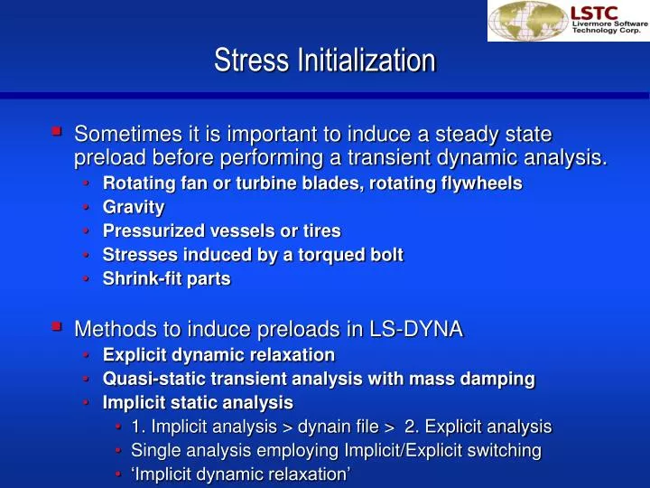
Stress Initialization. Sometimes it is important to induce a steady state preload before performing a transient dynamic analysis. Rotating fan or turbine blades, rotating flywheels Gravity Pressurized vessels or tires Stresses induced by a torqued bolt Shrink-fit parts

E N D
Stress Initialization • Sometimes it is important to induce a steady state preload before performing a transient dynamic analysis. • Rotating fan or turbine blades, rotating flywheels • Gravity • Pressurized vessels or tires • Stresses induced by a torqued bolt • Shrink-fit parts • Methods to induce preloads in LS-DYNA • Explicit dynamic relaxation • Quasi-static transient analysis with mass damping • Implicit static analysis • 1. Implicit analysis > dynain file > 2. Explicit analysis • Single analysis employing Implicit/Explicit switching • ‘Implicit dynamic relaxation’
Dynamic Relaxation (DR) • DR is an optional precurser transient analysis that takes place prior to the start of the regular transient analysis. • DR is typically used to preload a model before onset of transient loading. Preload stresses are typically elastic and displacements are small. • In DR, the computed nodal velocities are reduced each timestep by the dynamic relaxation factor (default = .995). Thus the DR solution is essentially a heavily damped transient solution. • The distortional kinetic energy is monitored. When this KE has been sufficiently reduced, i.e., the “convergence factor” has become sufficiently small, the DR phase terminates and the solution automatically proceeds to the transient analysis phase. • Alternately, DR can be terminated at a preset termination time.
Dynamic Relaxation DR converges • DR is typically invoked by setting parameter SIDR in any load curve (*DEFINE_CURVE) to 1 or 2. • Loads (curves) tagged for DR are ramped and then held constant until the DR solution converges • make sure convergence occurs on the loading ‘plateau’ • Maintain the load in subsequent transient analysis phase (use separate load curve without the ramp) SIDR = 1 (DR phase) SIDR = 0 (transient phase)
*CONTROL_DYNAMIC_RELAXATION *CONTROL_DYNAMIC_RELAXATION parameters • Iterations between convergence check (default=250) • Also controls output interval for DR • Convergence tolerance (default 0.001) • Ratio of distorsional KE at convergence to peak distorsional KE • Smaller value results in converged solution nearer to steady state but run will take longer to get there • Dynamic relaxation factor (default=0.995) • Reduction factor for nodal velocities each time step • If value is too small, model never reach steady state due to overdamping • Optional termination time for DR (default = infinity) • DR will stop if time reaches DRTERM even if convergence criterion not satisfied • Time step scale factor used during DR
*CONTROL_DYNAMIC_RELAXATION * IDRFLG • Set to 1, activates DR (not required if DR is activated with *DEFINE_CURVE) • Set to 2, will invoke a completely different and very fast initialization approach … Initialization by Prescribed Geometry. • Requires supplemental input file containing nodal displacements and rotations (“m=filename” on execution line). • Such a file “drdisp.sif” is written at conclusion of standard DR run. Required file format is I8,6E15 • If nodal rotations are not included in file, method is invalid for beams and shells. • LS-DYNA runs a short transient analysis of 100 timesteps to preload the model by imposing the nodal displacements and rotations. • Solution then proceeds with regular transient analysis. • Set to 5, activates implicit method for solution of preloaded state
Output related to Dynamic Relaxation • ASCII output files are NOT written during DR phase, e.g., GLSTAT, MATSUM, RCFORC, etc. • Binary database, d3drlf, is written by including command *DATABASE_BINARY_D3DRLF. Set output interval to 1. This will cause a state to be written each time convergence is checked during DR (as controlled by NRCYCK in *CONTROL_DYNAMIC_RELAXATION) • Plotting time histories from d3drlf with LS-PrePost allows user to confirm solution is near steady state • “relax” file is automatically written and contains record of convergence history. • “drdisp.sif” contains nodal displacements and rotations at conclusion of DR phase.
Loads during Dynamic Relaxation • Initial velocities are ignored during DR and are imposed at the commencement of the regular transient analysis. • Gravity loads and centrifugal loads (spinning bodies) are imposed using *LOAD_BODY_option. • LCID and LCIDDR are separate curves for transient phase and DR phase, respectively. • Stresses due to torqued bolts can be imposed using *LOAD_THERMAL_LOAD_CURVE. • Parts, e.g., bolts, which include coefficient of thermal expansion, e.g., via *MAT_4 or *MAT_ADD_THERMAL_EXPANSION will have thermal stresses imposed. • LCID and LCIDDR are separate curves for transient phase and DR phase, respectively. • Other load types or boundary conditions are applied during DR if SIDR flag in corresponding *DEFINE_CURVE is set to 1 or 2. Example: *LOAD_SEGMENT, *BOUNDARY_PRESCRIBED_MOTION. • Shrink-fit parts (see slide on *contact_interference)
Preloading a cross-section to a known stress • *INITIAL_STRESS_SECTION will preload a cross-section of solid elements to a prescribed stress value • Preload stress (normal to the cross-section) is defined via *DEFINE_CURVE (stress vs. time) • This curve is typically flagged with SIDR=1 so that dynamic relaxation is invoked for applying the preload • Stress should be ramped from zero • Physical location of cross-section is defined via *DATABASE_CROSS_SECTION • A part set, together with the cross-section, identify the elements subject to the prescribed preload stress • Contact damping and/or *damping_part_stiffness may be required to attain convergence during the dynamic relaxation analysis
*CONTACT_..._INTERFERENCE • For shrink-fit parts. The unstressed, pre-fit geometry which includes interferences (penetrations) is specified. • Contact forces are ramped up during DR to remove the interferences. • Shell thickness offsets are considered. • Specify the contact using two segment sets having correct orientation (or by a node set and a correctly oriented segment set). • To avoid sudden, large contact forces, the contact stiffness should be ramped. Contact stiffness scaling factors are specified via curves LCID1 (DR phase) and LCID2 (Transient phase). • Types: • *Contact_nodes_to_surface_interference • *Contact_one_way_surface_to_surface_interference • *Contact_surface_to_surface_interference
*CONTACT_..._INTERFERENCE Stiff. scale factor Stiff. scale factor Time Time Dynamic relaxation (LCID1) + Transient Phase (LCID2) 1.0 Stiff. scale factor 1.0 Time OR Transient Phase Only (LCID2) if LCID1=0 1.0
Transient Stress Initialization • As an alternative to using DR, in some cases the preload can be established in the early part of the regular transient simulation. • Not appropriate for problems whose transient response is driven by initial velocity. • Immediately ramp up preloads quasi-statically and then hold steady. • Use time-dependent mass damping (*DAMPING_GLOBAL) to impose near-critical damping until preload is established. • Drop damping constant to zero after preload is established and transient loading is ready to be applied. • Apply transient loads AFTER preload is established. • Use nonzero birthtime or nonzero arrival time for transient loads
Transient Stress Initialization Preload Transient Load Load Load t1 Time Time t2 Mass Damping Coef t1 t2 Time
Stress Initialization via Implicit Analysis • Recall that true static analysis is possible by invoking implicit analysis in LS-DYNA. Static analysis is well-suited to inducing preload. • Implicit analysis is invoked via the command *CONTROL_IMPLICIT_GENERAL. • Details of implicit analysis are beyond the scope of this course. See Appendix in the LS-DYNA User’s Manual.
Stress Initialization via Implicit Analysis • Approach 1: Two separate analyses. • Make an implicit (or explict) simulation of the preload. In the input deck specify *interface_springback_lsdyna. This creates an ASCII file called dynain when the simulation is finished. The dynain file contains keyword commands describing the deformed geometry, stresses, and plastic strains. Merge these commands into the original deck, deselect the implicit cards, modify the loads, and run a second, explicit simulation. • The dynain file does not include contact forces nor does it contain nodal velocities. Thus these quantities from the preload analysis do not carry over to the second analysis. • Taking data from the d3plot database, LS-PrePost can output a dynain file via Output > Format: Dynain Ascii > Write.
Stress Initialization via Implicit Analysis • Approach 2: Single, switched analysis. • Use one input deck where switching between implicit and explicit is determined by a curve. The abscissa of the curve is time and the ordinate is set to 1.0 for implicit and to 0.0 for explicit (curve is a step function). This switching is activated by setting IMFLAG at *control_implicit_general to -|curve ID|. Switching from one analysis to the other is seamless and has no CPU or I/O overhead.
Mapping Strains/Thicknesses from Metal Stamping Simulations Material Modeling for Metals
Need for strain/thickness mapping • Forming sheet metal components causes the material to harden • After Springback, the accumulated plastic strain increases the yield for any further loading • The assumption of constant thickness distribution may be inadequate for critical components as the thinning of sheet metal occurs during stamping operation • Initial mapping of plastic strain and thickness from one mesh to another is now handled trivially using LS-DYNA • Offers a method of mapping the strains and thickness that may be obtained from a metal stamping simulation • In v. 970, stresses and other history variables can also be mapped.
Need for strain/thickness mapping • From forming/springback simulation, write final stresses/strains/thickness at integration points using • *INTERFACE_SPRINGBACK_LSDYNA • this outputs a file “dynain” consisting of • *INITIAL_STRESS_SHELL • *INITIAL_STRAIN_SHELL • *ELEMENT_SHELL_THICKNESS • *NODE (deformed geometry) • The stamping simulation mesh may be much finer than the crash simulation mesh • Additionally, the stamped part may be oriented differently in the crash model • The mesh disparity as well as different orientation necessitates the need to map the variables
*INCLUDE_STAMPED_PART • Filename of “dynain” file containing information to be mapped • Crash Part ID • Variables to map • Thickness • Eff plastic strain • Strain tensor • Stress tensor • Orientation nodes from both models n2 stamp n1 n3 n3 crash n2 n1