Download

1 / 66
660 likes | 666 Views
Evaluation of a new tool for use in association mapping. Structure. Reinhard Simon, 2002/10/29. Software. Structure 2.0 http://pritch.bsd.uchicago.edu Pritchard JK, Stephens M, Donelly P (2000): Inference of population structure using multilocus genotype data. Genetics, 155 : 945-959.

E N D
Evaluation of a new tool for usein association mapping Structure Reinhard Simon, 2002/10/29
Software Structure 2.0http://pritch.bsd.uchicago.eduPritchard JK, Stephens M, Donelly P (2000):Inference of population structure using multilocus genotype data.Genetics, 155: 945-959
Associations – the ideal Cases Controls
Test for association A diploid locus: Pearsons Chi-square test
Associations – the less ideal Cases Controls
Associations – simple admixture Cases Controls
Associations – admixture complications Cases Controls
Associations – admixture complications Cases Controls High frequency of associated loci may indicate problems with underlying population structure (=stratification).
Associations – accounted for Cases Controls
Questions • Is there a stratification? • If so: - how many subpopulations - which individual belongs to which subpopulation
Test for stratification - principle Summarizing over all loci: • Xi is Chi-square at i-th locus • Null hypothesis: no differences between allele frequencies over all loci • df equal to sum of df at individual locus Pritchard: 1999
Test for stratification – ctd. Observations: • strong positive selection requires increase of #loci • subgroup specific markers decrease number of necessary loci Pritchard: 1999
How to group individuals? • Based on distance measures • Based on models
Pair wise distance measures Jaccard Nei & Li Sokal & Michener
Model based Bayesian inference • Bayesean statistics: Uncertainty is modeled using probabilities • probability statements are made about model parameters Advantages: • very general framework • assumptions are made explicit and are quantified
Bayesian inference – how? • Bayesian inference centers on the posterior distribution p(theta|X), e.g.a genetic model of the distribution of allele frequencies • However, analytic evaluation is seldom possible ....
Bayesian inference - methods Alternatives: • Numerical evaluation • approximation • simulation, e.g. Markov Chain Monte Carlo Methods
Simulation methods for Bayesian inference - general • Generate random samples from a probability distribution (e.g. normal) • Construct histogram • If sample is large enough, this allows to calculate mean, variance, ... • MCMC allows to generate large samples from any probability distribution
Markov Chain behaviour • Reaches an equilibrium (basic MCMC theorem) and • the present state depends only on the preceding: “The future depends on the past only through the present.”
MCMC - strengths • freedom in inference (e.g. simultaneous estimation, estimation of arbitrary functions of model parameters like ranks or threshold exceedence) • Coherently integrates uncertainty • Only available method for complex problems
MCMC – contra • computational intensive • requires often specialized software
Inferring population structure X = genotypes of sampled invidualsunknown:Z = population of originP = allele frequencies in all populationsQ = proportion of genome that originates from population k Pr(Z, P, Q|X) ~ Pr(Z) * Pr(P) * Pr(Q) * Pr(X|Z,P,Q) Solution:Using MCMC for Bayesian inference;simultaneous estimation of Q, Z and P.
Basic MCMC algorithm – no admixture (Q) Initialize:Random values for Z (pop), e.g. from Pr(z) = 1/k Repeat for m=1,2,...1. Sample P(m) from Pr(P|X, Z(m-1) (estimate allele frequencies) 2. Sample Z(m) from Pr(Z|X, P(m)) (estimate population of origin for each indiv.)
Basic MCMC algorithm – with admixture (Q) Initialize:Random values for Z (pop), e.g. from Pr(z) = 1/k Repeat for m=1,2,...1. Sample P(m), Q(m) from Pr(P, Q|X, Z(m-1) (estimate allele frequencies) 2. Sample Z(m) from Pr(Z|X, P(m), Q(m)) 3. Update alpha (admixture proportion)
Program – data types • marker: SNP, microsatellites AFLP, RFLP, ... (biallelic) • ploidy: >1 • extra optional information for inclusion: • prior knowledge on groups (e.g. geographic location) • genetic map location of marker
Example – S.t. tuberosum vs andigena Other:1st 30 genotypes from tuberosum 2nd 20 genotypes from andigena
Example – S.t. tuberosum vs andigena PNA: Estimation of k Simulation # k Pr(k)
Example – S.t. tuberosum vs andigena PNA: assignment 1 = tbr; 2 = adggenotypes #31-#3: adg from Indiagenotype #49: adg from Ecuador
Example – S.t. tuberosum vs andigena Parameter change: allow admixture Ancestry Model Info Use Admixture Model * Infer Alpha * Initial Value of ALPHA (Dirichlet Parameter for Degree of Admixture): 1.0 * Use Same Alpha for all Populations * Use a Uniform Prior for Alpha ** Maximum Value for Alpha: 10.0 ** SD of Proposal for Updating Alpha: 0.025Frequency Model Info Allele Frequencies are Independent among Pops * Infer LAMBDA ** Use a Uniform Lambda for All Population ** Initial Value of Lambda: 1.0
Example – S.t. tuberosum vs andigena Parameter change: allow admixture
Example – S.t. tuberosum vs andigena Parameter change: allow admixture
Example – S.t. tuberosum vs andigena Parameter change: allow admixture
Example – andigena K = 2
Example – andigena K = 3
Example – andigena K = 3