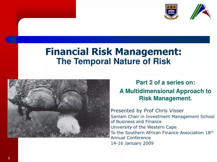
Financial Risk Management: The Temporal Nature of Risk

1. Financial Risk Management:The Temporal Nature of Risk Part 2 of a series on: A Multidimensional Approach to Risk Management. Presented by Prof Chris Visser Sanlam Chair in Investment Management School of Business and Finance University of the Western Cape To the Southern African Finance Association 18th Annual Conference 14-16 January 2009

2. Agenda • The Global Financial Crisis • Elements of Risk • The Dimensions of Risk • Revisiting the Square-Root-of-Time Rule • Brownian and Fractural Brownian Motion • The Hurst Coefficient and Memory Models • Incorporating Memory into Financial Models • Some Empirical Evidence

3. What does the following people have in common? • Botanist Robert Brown • Theorist Albert Einstein • Academics Myron Scholes and Fischer Black • Hydrologist Harold Edwin Hurst • Answer: • They basically faced the same problem. • All studied various processes that takes place over time.

4. The Global Financial Crisis: Quick perspective • Financial risk management has taken centre stage. • Quants have both been blamed for the crisis and hailed as the saviour of the financial system. • Herds of cloned quant analysts and financial engineers was let loose on Wall Street. • Some must take blame for the bull-run that ended in tears. • How did the ‘wiz-kids’ get it so wrong? • They neglect something critical from their market models. Why? • Financial engineers built models based on physical systems, not behavioural systems. • The dynamic nature of risk was not taken into account.

5. The changing risk profile of US Mortgage Debt

6. “We need new ways to measure risk!” * To manage you have to measure. To measure you have to understand. That may require a rethink! Textbook definitions and models such as CAPM must be revisited. Equating risk to volatility is assuming too much. * Business Report - December 23, 2008

7. Which is more risky?

8. Defining Financial Risk • Text book: Financial (Market) Risk is: • Risk of loss from changes in financial markets or conditions. • No reference to time or uncertainty. • A More Concise Definition: • A probability of a • loss (or below threshold returns) • during a certain time period. • 3 Elements to Risk • Uncertainty measured by probability. • A magnitude of loss (relative to something). • Time horizon. • Exposure is NOT Risk.

9. Have a Good Look at Risk!

10. The Multidimensional Nature of Risk Dimensions of Risk • Relevance • Direction • Distribution • Depth (Time horizon) • Memory • Attitude • Perspective • Association

11. The Square-Root-of-Time Rule • Risk increases with the root of the time horizon. • This rule is prevalent in finance and risk models • Value-at-risk: • VaR = -W(1-)t 0.5 • B-S Option Pricing • d1=[ln(S/X)+(r-q+0.5σ2)t]/(σt0.5) • d2=d1-σt0.5 • This rule is being applied blindly in finance based on the assumption that price movements follow the gBm process.

12. Observation Volume Brownian Motion

13. Fractural Brownian Motion (fBm) • Geometric Brownian Motion (gBm) • Relative change in price is a static mean times a time period plus a uncertain component with a Gaussian distribution time the square-root of the time period. • Alternative Model • Lift the assumption that sequential price movements are independent (No memory). • Log Returns follow a self-similar process called the Fractural (as in Mandelbrot) Brownian Motion. • Call for the introduction of additional model parameter call the Hurst Coefficient (H)

14. Implications of Autocorrelation in Returns • If we assume that the 1st and higher order auto-correlation of consecutive returns are not zero. • The square-root-of-time rule becomes: • Were ρnis the nth order autocorrelation coefficient of the stochastic process. • Problem with this model: • Higher order correlations are needed as parameters. • This is a discrete model. Fractions cannot be used.

15. The Hurst Coefficient for Self-Similar processes • Autocorrelation function time horizon (t) and the self similarity parameter Hurst Coefficient (H) or "index of dependence". • Limits for H: 0 H  1. • H = 0 : strong negative autocorrelation or ρ=-0.5 • Risk therefore not related to time • 0 < H < 0.5 : partial negative autocorrelation or -0.5 <ρ < 0 • Short-term memory model or reverting process. • H = 0.5 : zero autocorrelation or ρ=0 • Zero memory model. Random process. • 0.5 < H < 1 : partial positive correlation or 0 <ρ < 1 • long-term memory model. Trending process • H =1 indicates perfect positive correlation or ρ < 1. • Perfect memory. Linear process. No Risk

16. Fractural Brownian Motion Simulated

17. Advantages of Hurst in Self-Similar Process • The term horizon (t) is not limited to whole numbers. Any positive fraction or real number can be used • A requirement since the fBm is a continuous process. • The coefficient can easily be estimate using more that one method. • It fits neatly into currently used risk models. • Higher-order correlation coefficients are not required since this process is self-similar.

18. Estimating Hurst Coefficient (H) According to Beran(1994) the autocorrelation function of a such a self similar process is given as:[1] If t=1 then If ρ=ρ(1), then from previous equation we get It can be shown that the time risk relationship is: [1] Beran, J.

19. Estimating Hurst for SA Asset Classes Hurst Coefficient based on monthly returns From this table it is clear that: Equities do not have significant memory Bonds have short memory and Exchange rate and gold have long memory. This means that the risk projection over the medium- to long-term for these assets will be different and not follow the simple square-root-of-time rule.

20. Modification of Risk Models To compensate for autocorrelation of returns every should be replaced with Where the self similarity parameter of the self similar stochastic process. Using this modified square root of time rule, the basic VaR formula becomes: VaR = -W(1-)t H The d1 and d2 parameters in B-S option pricing model becomes: d1=[ln(S/X)+(r-q+0.5σ2)t]/(σtH) d2=d1-σtH

21. Modified Value at Risk (MVar) • The complete MVaR formula then becomes: where • W = the market value of the asset/portfolio • μ = the mean of the natural log returns • zc= the adjusted Gaussian critical value for probability (α) • σ = The standard deviation of the natural log of returns • H = Hurst coefficient of autocorrelation of log returns • t = Fraction of multiple of time horizon relative to frequency of returns.

22. Applying MVaR - Time Horizon is Important.

23. Conclusions • Markets (People) have memory. • Brownian motion process is assuming too much. • Self-similar process of a fractural Brownian is a more realistic choice. • Hurst coefficient (H) required to be added to models. • Option pricing and value-at-risk models can easily be modified with H. • Requires the estimation of an additional parameter. • H is easy to estimate. • Effort is justified for MT & LT market models.

24. Thank You Questions? Contact Details: Prof CF Visser: Cell: 083 675 6939 Email: cvisser@uwc.ac.za chris.visser@telkomsa.net