Download

1 / 25
250 likes | 347 Views
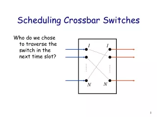
Scheduling Crossbar Switches. Who do we chose to traverse the switch in the next time slot?. 1. 1. N. N. History. [Karol et al. 1987] Throughput limited to by head-of-line blocking for Bernoulli IID uniform traffic.

E N D
Scheduling Crossbar Switches Who do we chose to traverse the switch in the next time slot? 1 1 N N
History • [Karol et al. 1987] Throughput limited to by head-of-line blocking for Bernoulli IID uniform traffic. • [Tamir 1989] Observed that with “Virtual Output Queues” (VOQs) Head-of-Line blocking is reduced and throughput goes up.
Basic Switch Model S(n) L11(n) A11(n) 1 1 D1(n) A1(n) A1N(n) AN1(n) DN(n) AN(n) N N ANN(n) LNN(n)
Some definitions 3. Queue occupancies: Occupancy L11(n) LNN(n)
A 1 2 B 3 C 4 D 5 E 6 F Finding a maximum size match • How do we find the maximum size (weight) match?
Network flows and bipartite matching A 1 2 B Finding a maximum size bipartite matching is equivalent to solving a network flow problem with capacities and flows of size 1. Sink t Source s 3 C 4 D 5 E 6 F
10 10 10 1 10 1 10 1 Network Flows a c Source s Sink t b d • Let G = [V,E] be a directed graph with capacity cap(v,w) on edge [v,w]. • A flow is an (integer) function, f, that is chosen for each edge so that • We wish to maximize the flow allocation.
10 10 10 1 10 1 10 1 a c 10, 10 Source s Sink t 10, 10 1 10, 10 10 1 10 b d 1 Flow is of size 10 A maximum network flow exampleBy inspection a c Source s Sink t b d Step 1:
Not obvious Maximum flow: a c 10, 9 Source s Sink t 10, 10 1,1 10, 10 1,1 10, 2 b d 10, 2 1, 1 Flow is of size 10+2 = 12 A maximum network flow example Step 2: a c 10, 10 Source s Sink t 10, 10 1 10, 10 1 10, 1 b d 10, 1 1, 1 Flow is of size 10+1 = 11
Ford-Fulkerson method of augmenting paths • Set f(v,w) = -f(w,v) on all edges. • Define a Residual Graph, R, in which res(v,w) = cap(v,w) – f(v,w) • Find paths from s to t for which there is positive residue. • Increase the flow along the paths to augment them by the minimum residue along the path. • Keep augmenting paths until there are no more to augment.
Example of Residual Graph a c 10, 10 10, 10 1 10, 10 s t 10 1 10 b d 1 Flow is of size 10 Residual Graph, R res(v,w) = cap(v,w) – f(v,w) a c 10 10 10 1 s t 10 1 10 b d 1 Augmenting path
Example of Residual Graph Step 2: a c 10, 10 s t 10, 10 1 10, 10 1 10, 1 b d 10, 1 1, 1 Flow is of size 10+1 = 11 Residual Graph a c 10 s t 10 10 1 1 1 1 b d 9 1 9
Complexity of network flow problems • In general, it is possible to find a solution by considering at most VE paths, by picking shortest augmenting path first. • There are many variations, such as picking most augmenting path first. • Best Algorithm based on work by Dinic. • Complexity: O(nm)
A 1 2 B 3 C 4 D 5 E 6 F Finding a maximum size match • How do we find the maximum size (weight) match?
Network flows and bipartite matching A 1 2 B Finding a maximum size bipartite matching is equivalent to solving a network flow problem with capacities and flows of size 1. Sink t Source s 3 C 4 D 5 E 6 F
Network flows and bipartite matchingFord-Fulkerson method Residual Graph for first three paths: A 1 2 B t s 3 C 4 D 5 E 6 F
Network flows and bipartite matching Residual Graph for next two paths: A 1 2 B t s 3 C 4 D 5 E 6 F
Network flows and bipartite matching Residual Graph for augmenting path: A 1 2 B t s 3 C 4 D 5 E 6 F
Network flows and bipartite matching Residual Graph for last augmenting path: A 1 2 B t s 3 C 4 D 5 E 6 F Note that the path augments the match: no input and output is removed from the match during the augmenting step.
Network flows and bipartite matching Maximum flow graph: A 1 2 B t s 3 C 4 D 5 E 6 F
Network flows and bipartite matching Maximum Size Matching: A 1 2 B 3 C 4 D 5 E 6 F
Complexity of Maximum Matchings • Maximum Size Matchings: • Algorithm by Dinic (~1970) O(n1/2m) • Maximum Weight Matchings (assignment problem) • Algorithm by Kuhn (1955) O(N3) • In general: • Hard to implement in hardware • Slooooow.
Properties of LPF • LPF is stable for all admissible Bernoulli traffic. • An LPF match is a maximum size match. • How can this be stable?