Download
1 / 11
110 likes | 225 Views
Note. The animations in these slides have been removed. For the full set of slides, including animations, download http://www.cs.ucl.ac.uk/staff/D.Wischik/Talks/switch-infocom.zip. optimal scheduling algorithms for input-queued switches. Devavrat Shah, MIT Damon Wischik, UCL.

E N D
Note. The animations in these slides have been removed. For the full set of slides, including animations, download http://www.cs.ucl.ac.uk/staff/D.Wischik/Talks/switch-infocom.zip optimal scheduling algorithmsfor input-queued switches Devavrat Shah, MIT Damon Wischik, UCL
Input-queued crossbar switch • The matching (or scheduling) algorithmdecides which inputs to match with which outputs • What is a good scheduling algorithm? • What is the quality of service / queueing performance? • What is the relationship between scheduling and performance?
Example: Serve the longer queue second queue size first queue size
Example: Serve the longer queue • The system is basically one-dimensional + noise • If we keep track of the total queue size W, we can deduce the individual queue sizesQ1≈ Q1≈ W/2 • This relationship does not depend on the arrival rates (so long as the system is stable) second queue size first queue size
Example: Serve the longer queue • Another way to visualize this relationship is to plot both • the actual queue sizes • the queue sizes estimated from the workload W, Q1=Q1=W/2 • These agree almost perfectly second queue size firstqueue secondqueue totalworkload first queue size
Terminology • State space collapse (SSC) • the fact that the vector of queue sizes Q can be written as a function of the workload W, Q=ΔW • Workload • a carefully chosen sum of queue sizes • Lifting map • Δ • Collapsed (or invariant) space • { (Q1, Q2) : Q1= Q2 } • more generally, the set of achievable Q=ΔW, as W varies
Input-queued switches have state space collapse! • For a n×n switch there are n2 queues to keep track of • The workload vector lists the total queue size for each input port and for each output port, and it has dimension 2n-1 • The lifting map Δ depends on the scheduling algorithm • Here I’ve illustrated the maximum weight matching scheduler: • at each time step, choose a set of queues to serve so that the sum of their queue sizes is as large as possible
Technical details • Method • write down differential equations describing the system, i.e. a fluid model • use combinatorial techniques to prove convergence, and to characterize the fixed points • use heavy traffic queueing theory to show that as the load on the switch increases, fluctuations in Q away from ΔW become negligible compared to Q • Lifting map: for arrival rate matrix λ, q=Δw is the unique solution to
Why is this useful? (I) • We’ve shown that Q=ΔW • Once we’ve found Δ it’s easy to work out if any queues are persistently small, i.e. guaranteed good quality of service • We can also see if giving priority to some queues has a negative impact on others
Why is this useful? (II) • We’ve shown that Q=ΔW • W is easier to reason about than Q • In those states where every queue is non-zero, the switch is work-conserving (i.e. no service is wasted) • It’s therefore useful to look at the space {W : ΔW >0} and to choose the scheduling algorithm to make this as big as possible • We’ve used this to conjecture an optimal scheduling algorithm • i.e. one which never wastes service because of poor scheduling(in a stochastic limit sense) • At each timestep, it considers all max-size matchings, and chooses one with maximum log-weight
Conclusion • We have reduced the problem of analysing scheduling algorithms to questions about the algebra of Δ • It’s hard algebra! • So far we only know Δ for a small class of algorithms, variations on maximum-weight matching • The same approach works for any generalized switch, e.g. schedulers in wireless base-stations