Download
1 / 50
500 likes | 594 Views
Chapters 14 and 15 – Linear Regression and Correlation. Contingency tables are useful for displaying information on two qualitative variables. Scatter plots are useful for displaying information on two quantitative variables.

E N D
Contingency tables are useful for displaying information on two qualitative variables
Scatter plots are useful for displaying information on two quantitative variables.
What type of relationship is present in the following scatter plot? No relationship Linear relationship Quadratic relationship Other type of relationship
What type of relationship is present in the following scatter plot? No relationship Linear relationship Quadratic relationship Other type of relationship
What type of relationship is present in the following scatter plot? No relationship Linear relationship Quadratic relationship Other type of relationship
What type of relationship is present in the following scatter plot? No relationship Linear relationship Quadratic relationship Other type of relationship
What type of relationship is present in the following scatter plot? No relationship Linear relationship Quadratic relationship Other type of relationship
What type of relationship is present in the following scatter plot? No relationship Linear relationship Quadratic relationship Other type of relationship
What type of relationship is present in the following scatter plot? No relationship Linear relationship Quadratic relationship Other type of relationship
We can quantify how strong the linear relationship is by calculating a correlation coefficient.The formula is:It is easier to let technology do the calculation!
We can quantify how strong the linear relationship is by calculating a correlation coefficient.It is easier to let technology do the calculation!You have multiple options: • Calculator • Minitab • Excel • Websites
Calculation exampleCorrelation Coefficient = -0.492Correlation Coefficient is abbreviated by r.r = -0.492 x y 5 7 2 6 3 8 6 4 5 5 4 6 2 6
TI Calculator: Type x data into L1 and y data into L2 then go to VARS -> Statistics -> EQ -> rr = -0.492Note: it does not matter which is the x data and which is the y data for computing r. x y 5 7 2 6 3 8 6 4 5 5 4 6 2 6
x y 2 14 14 10 57 28 14 16 23 16 56 18 8 1 Consider the following data: r = - 0.734 r = 0.538 r = 0.734 r = 0.466 r = - 0.538
x1 x2 0 -4 8 -6 7 -8 9 -9 5 -5 8 -8 8 -7 6 -9 Consider the following data: r = - 0.034 r = - 0.724 r = - 0.545 r = - 0.983 r = - 0.241
If then there is a negative relationship between the two variables • If then there is a positive relationship between the two variables • r only measures a linear relationship • The greater , the stronger the relationship Properties of the Correlation Coefficient
The correlation coefficient is 0.734There is a positive relationship x y 2 14 14 10 57 28 14 16 23 16 56 18 8 1
The correlation coefficient is - 0.724There is a negative relationship x1 x2 0 -4 8 -6 7 -8 9 -9 5 -5 8 -8 8 -7 6 -9
r = - 0.821 r = - 0.759 r = 0.388 r = 0.674 r = 0.983 r = 0.983 Guess the correlation
r = 0.121 r = 0.372 r = 0.644 r = 0.865 r = 0.978 r = 0.865 Guess the correlation
r = 0.372 r = 0.522 r = 0.644 r = 0.865 r = 0.978 r = 0.522 Guess the correlation
r = - 0.034 r = - 0.299 r = - 0.438 r = - 0.601 r = - 0.894 r = - 0.601 Guess the correlation
r = - 0.004 r = - 0.156 r = - 0.441 r = - 0.699 r = - 0.923 r = - 0.156 Guess the correlation
r = 0.7484 r = 0.3156 r = 0.0116 r = - 0.2994 r = - 0.6235 r = 0.0116 Guess the correlation
r = 0.7484 r = 0.2676 r = 0.0018 r = - 0.1944 r = - 0.7588 r = 0.0018 Guess the correlation
Fill in the blank: If one variable tends to increase linearly as the other variable increases, the variables are __________ correlated. Positively Negatively Not
Fill in the blank: If one variable tends to increase linearly as the other variable decreases, the variables are __________ correlated. Positively Negatively Not
If there is a correlation (relationship) between two variables, it does not necessarily mean there is a causal relationship between the two variables (one variable affects the other).
If there is a correlation (relationship) between two variables, it does not necessarily mean there is a causal relationship between the two variables (one variable affects the other)
The correlation coefficient of this data set is closest to what value? -0.999 0.999 0.099 -0.099 Nobel Prize and McDonalds data set
The correlation between the number of Nobel Prizes awarded and number of McDonald’s Restaurants for select countries is strong. Therefore, we can correctly conclude that if a country were to build more McDonald’s Restaurants its inhabitants would be more likely to receive Nobel Prizes. True False
A confounding variable is a variable that is not accounted for that can affect both variables being studied. Nobel Prize and McDonalds data set
Recall the equation of a line is: where m is the slope of the line and b is the y intercept.In statistics we use this notation: where is the slope and is the yintercept. The values of and are unknown and must be estimated from the data.
The values of and are unknown and estimated using a method called “least squares.” This method picks the line that minimizes the sum of the squared errors of all the data points.What is an error?
An error is the vertical distance between a data point and the line and is abbreviated as ε
The method of least squares picks the line that results in this being the smallest: .
We will let computes calculated the line of best fit or the least squares line because it requires multivariate calculus.
The regression line below is a poor fit of the data and results in high error.
The regression line below is a better fit of the data and results in lower error.
The regression line below is the line of best fit or the least squares line.
Review of properties of a line! Consider: where x measures time in hours and y measures distance in miles. The interpretation if the slope is? An increase of 1 hour results in an increase of 2.4 miles. A decrease of 1 hour results in an increase of 2.4 miles. A decrease of 2.4 miles results in a decrease of 1 mile. An increase of 2.4 miles results in a decrease of 1 mile.
A study looked at the weight (in hundreds of pounds) and mpg of 82 vehicles. Following is the scatter plot:
The line of best fit is: MPG = 68.2 - 1.11 Weight. What does the slope tell us? An increase in mpg of 1 results in an increase in weight of 111 pounds. A decrease in mpg of 1 results in an increase in weight of 111 pounds. An increase in weight of 100 pounds results in a decrease in gas mileage of 1.11 mpg. An increase in weight of 100 pounds results in an increase in gas mileage of 1.11 mpg.
A car with a weight of 0 lbs gets 68.2 mpg A car with a weight of 100 lbs gets 68.2 mpg A car with a weight of 1000 lbs gets 68.2 mpg A car with a weight of 2000 lbs gets a 68.2 mpg The line of best fit is: MPG = 68.2 - 1.11 Weight. What does the y-intercept tell us?
Consider the following data set and graph. The graph is of this data. True False
A direct relationship means an increase in one variable results in an increase in the other. This is also a positive correlationAn inverse relationship means an increase in one variable results in a decrease in the other. This is also a negative correlation
There is a negative correlation between the two variables which indicates a direct relationship between femur length and horse height. • There is a positive correlation between the two variables which indicates an inverse relationship between femur length and horse height. • There is a negative relationship between the two variables which indicates an inverse relationship between femur length and horse height. • There is a positive relationship between the two variables which indicates a direct relationship between femur length and horse height. • None of the above