Download
1 / 31
320 likes | 326 Views
Metapopulation Biology What is a metapopulation?

E N D
Metapopulation Biology What is a metapopulation? According to Levins’ original formulation, a metapopulation is a “population of populations”. It is a set of populations located in/on spatially distinct habitats (islands, patches) that exchange individuals with (reasonable) likelihoods of immigration between populations and of extinction of individual populations. Drawing from the text: “metapopulations are regional assemblages of plant or animal species, with the long term survival of the species depending on a shifting balance between local extinctions and re-colonization in a patchwork of fragmented landscapes.
The basic models make a number of unrealistic assumptions, though the results are still valuable. • All patches are equally accessible to colonists from any other patch, i.e. the patches are equidistant. If there are more than 3 patches, how can this be? • Areas of patches are unimportant. We are interested only in whether a patch is occupied or not. From what you already know about the probability of extinction, isn’t population size important? • The qualities of all patches are identical. Is this likely?
What is usually of interest in basic metapopulation models is whether persistence of the metapopulation greatly exceeds the expected persistence of individual local populations. In other terms, whether probability of regional extinction is much lower than the probability of local extinction. There are various ‘kinds’ of metapopulations. We’ll look at them in ‘historical’ order.
Island-mainland (Island biogeography) models You should have encountered the basics of this model in Ecology. MacArthur and Wilson (1963, 1967) proposed a model for isolated islands that determined species diversity on them resulting from a balance between immigration onto the islands and extinction on them. The number of species occurring on an island was determined by the area of the island. The equation for that number also includes a constant set by the dispersal ability of the taxonomic group in question. The equation: S = CAz In this model there is a source pool of species from which colonists come – the mainland.
If this equation is transformed by taking logs, the resulting relationship between (log) species number and (log) area is linear… Log S = log C + z log A There is a classic example, cited in almost every text, of the species-area curve for reptiles on Caribbean islands…
The slope z has been a point of great interest. Most species-area curves seem to have slopes of about 0.25. There is an underlying theoretical reason for that. In Ecology you may have also encountered the Preston log normal abundance curve for species in a community. It suggests that a plot of the log of individual species abundance (usually plotted in base 2) versus the number of species with those abundances should follow a normal curve, as shown for moths captured at a light trap in England:
Much different slopes have been observed. The question is why? Much lower slopes have been found when the patches or islands are not really isolated, for example when larger and larger areas are sampled from a mainland area as if they were separate. Much larger slopes have been observed when unexpectedly high habitat diversity occurs within patches, or, in one example, when pollution may have reduced species interactions among populations in patches. There is, once more, a classic plot, comparing bird diversity in patches on New Guinea with that found on isolated oceanic islands nearby…
What determines the number of species is the balance between immigration and extinction. Over time the immigration rate (beginning with a bare island) declines from an initially high rate to potentially reach zero when all species from the mainland pool have reached the island. Meanwhile, as species accumulate, extinctions occur due to chance events when population(s) are small or to interactions among species as more are present.
The standard depiction of this relationship is: When immigration and extinction rates are equal, an equilibrium is reached. The number of species doesn’t change, but there is still turnover. There are changes in the names on the list.
There is one characteristic of the mainland-island metapopulation model that may not be obvious: since there is an unending source of potential colonists from the mainland, the equilibrium occupancy of patches is greater than zero – the island metapopulation should never go regionally extinct. That is not necessarily true of the Levins (or classical) metapopulation. In the Levins model there are only isolated patches, with no mainland source. Whether the metapopulation persists or not is determined by the balance between colonization and extinction rates on patches. Of the total number of patches available in the region, the number currently occupied by this species is called P. By this definition of P, 0 P 1.
The value of P is determined by a balance between immigration, I, which leads to the occupation of previously unoccupied patches, and local extinction, E, which causes a previously occupied patch to become unoccupied. There are close analogies to both the basic equation for exponential growth and the basic equation of island biogeography in this formulation. dP/dt = I - E Immigration is determined by a characteristic rate, c, times the number of occupied sites that can provide immigrants (P), but can only occur onto unoccupied sites (1-P). Extinction is set by a characteristic rate and the number of occupied sites at which extinction could occur. Thus: dP/dt = cP(1-P) - P
What we are really interested in from this model is the equilibrium occupancy of patches. We can find the equilibrium if we set dP/dt to 0 and solve. cP(1-P) = P P = 1 – /c Unless c > an uninteresting equilibrium of regional extinction results. If c > then there is a positive equilibrium and persistence of the metapopulation. It diesn’t matter what the initial proportion of sites occupied is, the metapopulation will ‘converge’ on a proportion determined by whatever the fixed and c are.
There is a useful parallel to growth equations that can be drawn from this. c, the colonization rate, is like a birth rate; is like a death rate. In this notion of a parallel, r = c - and carrying capacity is 1 – /c. As a parallel to the logistic equation: dP/dt = (c- ) P (1 – [P/(1 - /c)] The same parabolic graph that was useful in evaluating the effect of harvesting for the logistic model can be used to evaluate the effects of changes in colonization and extinction rates on equilibrium occupancy…
How can we compare the probability of regional extinction in a metapopulation versus one which is not subdivided? As a first step, we can assess the probability of regional extinction using the basic rules for combinations of independent events. Local populations may have fairly large probabilities of extinction, even when probabilities are measured on a short term basis, i.e. probabilities for a time period of one year. What if the probability of local extinction in a single year is 0.7 (pe). Then (1-pe) is the probability of population persistence. If we want to know what the probability of persistence is over a two year period, it is: P2 = (1-pe)(1-pe) = (1-pe)2 or, for an y year period Py = (1-pe)y
The probability of persistence for a single local population can become very small over very few years. However, what happens when we consider a group of local populations which comprise a metapopulation? Assume that patches are identical, with identical probabilities of local extinction. If there are n such populations functioning independently with regard to extinction, then the probability of all going extinct in any one year is: P(0)n = (pe)n And of persistence is: Pn = 1- (pe)n Now with only a few local populations as components of the metapopulation, the probability of persistence can be quite high, even with a high probability of local extinction in each of the component populations.
This all works based on the assumption that processes in separate populations are asynchronous. Remember what happened when time lags were important, and produced chaotic behaviour in population size? That chaotic behaviour can be mitigated by exchange between component populations of a metapopulation. Thus far we’ve looked at two kinds of metapopulations: mainland-island and Levins’ classic metapopulations. It’s time to move on to the third type,
Source-sink metapopulations There is a partial similarity to island-mainland models here. Though there is no mainland, there are patches with superior habitat and consistent growth rates > 0. They are sources of colonists. Those colonists move to patches where conditions are not so positive, and growth rates average < 0. They are sinks. Populations would not persist there without colonists from sources. What happens in sink populations? Without new immigrants from source populations, they would go locally extinct. However, immigrants arrive more-or-less frequently. Those immigrants prevent local extinction. This is called the rescue effect.
The text distinguishes between a ‘true sink’ population that would decline to extinction without rescue from a source population and a ‘pseudo-sink’ population that would decline to a clearly lower equilibrium size in the absence of a source. In real world, field situations there is no easy way to distinguish the two types of sink populations.
If you remember the MacArthur-Wilson model of island biogeography, you should see a great deal of similarity between source-sink metapopulations and the island-mainland model of island biogeography. The mainland (e.g. New Guinea for bird populations) is a source, and the isolated islands are likely to be sinks, at least in the long run (and particularly for distant, isolated islands). A neat example of a real world source- sink system is rare tropical tree species in the forests of Barro Colorado island. The distribution of abundance among species is a very good fit to the Preston log-normal.
There are usually more rare than common species, and here, if there is a deviation from the log-normal, it is to have even more rare species than predicted by the theoretical distribution of abundances. Quoting from the summary of the paper: “Many (at least one third) of the rare species (fewer than 50 total individuals) do not appear to have self-maintaining populations in the plot [50 hectares with approximately 238,000 individual trees and shrubs]. Their presence appears to be the result of immigration from population centers outside the plot, and their numbers are probably kept low by a combination of unfavorable regeneration conditions, lack of appropriate habitat, or both, in the plot” (Hubbell and Foster 1986)
The last type of metapopulation takes two forms, linked in the text. The first is described as a non-equilibrium metapopulation. It could probably be better described as a 0 equilbrium form. The rate of extinction exceeds the rate of colonization. Unless something changes (e.g. rescue from some source), the equilibrium state is regional extinction. The second form is called a patchy population. Here the opposite is occurring, colonization (or migration) rate is so high that the population is not really subdivided effectively into a metapopulation.
When metapopulation models are made more realistic, particularly with regard to space, one is moved back in the direction of studies associated with the MacArthur-Wilson island biogeography approach. What determines the likelihood of a patch being colonized, or, alternatively, of a propagule reaching the patch? How far away are sources? What are the dispersal characteristics of potential colonists? These questions were initially studied by Diamond in modeling the probabilities of birds colonizing New Guinea satellite islands. The important characteristics were the number of dispersers and the distance to the island, embodied in the equation: C = e-d
C is the number of propagules reaching the isolated patch • is the number of propagules produced by the source • is the characteristic describing the dispersal function, and d is the distance between source and isolated patch. Diamond also recognized that patch area makes a difference. Larger patches are more likely to be found (and, in island biogeography, can support a larger number of species). Diamond also recognized that different species have differing dispersal characteristics and tendencies to disperse.
From all this, he constructed incidence functions. Some species, called super tramps, are very likely to disperse, can move long dsitances, and are thus early colonists, as well as the most likely to reach very isolated patches. They tend to be weak competitors, and disappear from patches when they are colonized by species more adapted to diverse communities. There are a range of different groups of tramp species, not such extreme dispersers, but even they eventually are displaced by species with limited dispersal capability, but strong ability to compete for resources. Hanski and his collaborators, critical in the development of metapopulation theory, turned this basic idea on its head, and developed incidence functions that assess the long-term probability of a patch being occupied.
One of the key questions (particularly to conservation biologists) is what conditions lead to long-term survival of a metapopulation. To have a metapopulation survive at least 100x the expected survival time for a local component population, it has been found that: Where P is the equilibrium proportion of patches occupied and H is the total number of patches available. The last thing to consider is data that supports the metapopulation approach…
First is a basically mainland-island example of the checkerspot butterfly, Euphydras edita, which lives in the area around San Francisco, and is monophagous, at least as a caterpillar, using an annual plantain, Plantago erecta, as both a site for egg laying and a food source. This plantain grows on serpentine rock outcrops. There are many small outcrops, and one large one, called Morgan Hill. There are estimates of hundreds of thousands of butterflies on Morgan Hill, but only a shifting mosaic of presence on the other sites. The causes of local extinctions vary. Many local extinctions occurred during an extended severe drought that lasted from 1975-7. The figure on the next slide maps the outcrops around Morgan Hill, and indicates a few recent events for the metapopulation.
Maps from other sources make it apparent that isolation (distance from Morgan Hill) is an important factor. Most colonization events recorded occurred on outcrops close to the source 'mainland'. Extinction events are more widely distributed.
A second example is carabid ground beetles. They have been studied for more than 3 decades in the Netherlands. Radioactive tags indicate they remain fairly localized, moving less than 100 m per day. As a result, the relative isolation of populations required for effective metapopulation dynamics is likely, even over short distances. The figure that follows shows dynamics in two different beetle species. The upper panel shows numbers of individuals in different component populations of Pterostichus versicolor. The different populations fluctuated asynchronously, so that when one population declined in size, another was likely to be increasing. Sources were increasing populations likely to be throwing off emigrants. The sinks were declining populations; extinction was prevented by immigrants from source populations.
The lower panel shows the dynamics of component populations in a different species, Calathus melanocephalus. There is a much greater synchrony among components. When one population is declining, so do most, if not all others. Whatever caused the declining periods, they drove populations locally extinct; since there were no source populations providing emigrants to colonize sink populations. Local extinction (and even regional extinction) is much more likely when populations within a metapopulation function synchronously.
References Den Boer, P. 1981. On the survival of populations in a heterogeneous and variable environment. Oecologia, 50:39-53. Diamond, J.M. 1975a. Assembly of species communities. In M.L. Cody and J.M. Diamond, eds. Ecology and Evolution of Communities. pp.342-444. Belknap Press, Cambridge, MA Diamond, J.M. 1975b. The island dilemma: Lessons of modern biogeographic studies for the design of natural reserves. Biol. Conserv. 7:129-146. Hanski, I. 1999. Metapopulation Ecology. Oxford Univ. Press, Oxford. Harrison, D., D.D. Murphy and P.R. Ehrlich. 1988. Distribution of the bay checkerspot butterfly, Euphydras editha bayensis: evidence for a metapopulation model. Amer. Natur. 132:360-382. Hubbell, S.P. and R. Foster. 1986. Commoness and rarity in a Neotropical forest: implications for tropical tree conservation. Pp. 205-231 in M.E. Soule, ed. Conservation Biology: The Science of Scarcity and Diversity. Sinauer Assoc., Sunderland, MA.