Download
1 / 28
280 likes | 444 Views
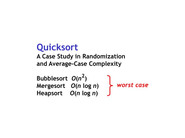
Quicksort A Case Study in Randomization and Average-Case Complexity Bubblesort O ( n ) Mergesort O ( n log n ) Heapsort O ( n log n ). 2. worst case. Interesting Fact

E N D
Quicksort A Case Study in Randomization and Average-Case Complexity Bubblesort O(n) Mergesort O(n log n) Heapsort O(n log n) 2 worst case
Interesting Fact Every comparison-based sorting algorithm must make at least n log n comparisons on inputs of length n in the worst case! It must distinguish between n! ~ 2 possible input permutations, and the decision tree must have depth at leastn log n to have that many leaves. n log n n log n n log n n! ~ 2
QUICKSORT—a very fast sorting method • Worst case O(n ); so what's so quick about it? • It's O(n log n) expected time • It's got a very small constant 2
Idea • To sort the subrange v[p]…v[r]: • let a = v[p]; a is called the pivot • move elements a to the front • move elements a to the back • let q be such that all v[p]…v[q] a and all v[q+1]…v[r] a; recursively sort v[p]…v[q] and v[q+1]…v[r]
;; sort the subrange of vector v ;; from p to r, inclusive (define (qsort! <function>) (method ((v <vector>) (p <integer>) (r <integer>)) (when (< p r) (bind (((q <integer>) (partition! v p r))) (qsort! v p q) (qsort! v (inc q) r)))))
;; move small elements to beginning of interval ;; large elements to end of interval ;; return max bound of lower subinterval (define (partition! <function>) (method ((v <vector>) (p <integer>) (r <integer>)) (bind (((pivot <number>) (index v p))) (bind-methods ((count-down ((k <integer>)) (if (<= (index v k) pivot) k (count-down (dec k)))) (count-up ((k <integer>)) (if (>= (index v k) pivot) k (count-up (inc k)))) (iter ((i <integer>) (j <integer>)) (cond ((< i j) (swap! v i j) (iter (count-up (inc i)) (count-down (dec j)))) (else: j)))) (iter (count-up p) (count-down r))))))
;; swap two elements of an array in place (define (swap! <function>) (method ((v <vector>) (i <integer>) (j <integer>)) (bind (((temp <number>) (index v i))) (index-setter! i v (index v j)) (index-setter! j v temp))))
3 5 4 7 0 8 2 1 9 6 ^ ^ p r
3 5 4 7 0 8 2 1 9 6 ^ ^ i j
3 5 4 7 0 8 2 1 9 6 ^ ^ i j
1 5 4 7 0 8 2 3 9 6 ^ ^ i j
1 5 4 7 0 8 2 3 9 6 ^ ^ i j
1 2 4 7 0 8 5 3 9 6 ^ ^ i j
1 2 4 7 0 8 5 3 9 6 ^ ^ i j
1 2 0 7 4 8 5 3 9 6 ^ ^ i j
1 2 0 7 4 8 5 3 9 6 ^ ij
1 2 0 7 4 8 5 3 9 6 ^ ^ j i
1 2 0 7 4 8 5 3 9 6 ^ ^ j j+1
1 2 0 7 4 8 5 3 9 6 ^ ^ ^ ^ p q q+1 r
0 1 2 3 4 5 6 7 8 9 ^ ^ ^ ^ p q q+1 r
Running time depends on how • balanced the partitions are • BEST CASE • pivot is always the median of the interval • we cut the array in half in each iteration • T(n) = O(n) + 2T(n/2) = O(n log n) • WORST CASE • pivot is always the smallest element of the interval • gives a 1:n-1 split (example: [1,2,3,4,5]). • T(n) = T(n-1) + O(n) = O(n^2)
Best case Worst case Running time ~ n·depth of tree
Suppose the partition produces a 9:1 split 90% in one half, 10% in the other. Still O(n log n) ! T(n) = T(0.9 n) + T(0.1 n) + O(n) = O(n log n)
Quicksort will occasionally have bad partitionings at some stages, but it's very unlikely to have enough of them to matter. • It can be shown that, if we assume the input is random and uniformly distributed (all permutations equally likely), then the probability that the partition is better than a:1-a is 1-2a (0 < a 1/2). • For example, if we want a 9:1 or better split, then we compute: • a=0.1 • probability = 1-2(0.1) = 80%
So we would expect about 4 out of every 5 arrays to be 9:1 or better. Even if the other arrays are utterly useless, this is still exponential decay, and we still get O(n log n).
DEFINITION The expected running time of an algorithm is a function of n giving the average running time on inputs of length n. T(x) = running time on input x = probability that x occurs among inputs of length n THEOREM Assuming the elements of the input vector are distinct and all permutations are equally likely, the expected running time of quicksort is O(n log n). Pr (x) n E(n) = T(x)· Pr (x) n |x|= n
Q. How reasonable is it to assume the input is random? • A. Not very. • worst case = input is already sorted • choosing v[p] as pivot guarantees a 1:n-1 split • this happens a lot in real life
Trick: scramble the input! ;; scramble a vector (define (scramble! <function>) (method ((v <vector>)) (bind-methods ((scram! ((i <integer>)) (cond ((< i (length v)) (swap! v i (random i)) (scram! (inc i)))))) (scram! 0))))