Download
1 / 82
860 likes | 906 Views
Introduction to Management Science 8th Edition by Bernard W. Taylor III. Chapter 15 Forecasting. Chapter Topics. Forecasting Components Time Series Methods Forecast Accuracy Time Series Forecasting Using Excel Time Series Forecasting Using QM for Windows Regression Methods.

E N D
Introduction to Management Science 8th Edition by Bernard W. Taylor III Chapter 15 Forecasting Chapter 15 - Forecasting
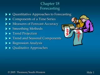
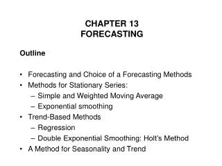
Chapter Topics • Forecasting Components • Time Series Methods • Forecast Accuracy • Time Series Forecasting Using Excel • Time Series Forecasting Using QM for Windows • Regression Methods Chapter 15 - Forecasting
Forecasting Components • A variety of forecasting methods are available for use depending on the time frame of the forecast and the existence of patterns. • Time Frames: • Short-range (one to two months) • Medium-range (two months to one or two years) • Long-range (more than one or two years) • Patterns: • Trend • Random variations • Cycles • Seasonal pattern Chapter 15 - Forecasting
Forecasting Components Patterns (1 of 2) • Trend - A long-term movement of the item being forecast. • Random variations - movements that are not predictable and follow no pattern. • Cycle - A movement, up or down, that repeats itself over a lengthy time span. • Seasonal pattern - Oscillating movement in demand that occurs periodically in the short run and is repetitive. Chapter 15 - Forecasting
Forecasting Components Patterns (2 of 2) Figure 15.1 Forms of Forecast Movement: (a) Trend, (b) Cycle, (c) Seasonal Pattern, (d) Trend with Seasonal Pattern Chapter 15 - Forecasting
Forecasting Components Forecasting Methods • Times Series - Statistical techniques that use historical data to predict future behavior. • Regression Methods - Regression (or causal ) methods that attempt to develop a mathematical relationship between the item being forecast and factors that cause it to behave the way it does. • Qualitative Methods - Methods using judgment, expertise and opinion to make forecasts. Chapter 15 - Forecasting
Forecasting Components Qualitative Methods • Qualitative methods, the “jury of executive opinion,” is the most common type of forecasting method for long-term strategic planning. • Performed by individuals or groups within an organization, sometimes assisted by consultants and other experts, whose judgments and opinion are considered valid for the forecasting issue. • Usually includes specialty functions such as marketing, engineering, purchasing, etc. in which individuals have experience and knowledge of the forecasted item. • Supporting techniques include the Delphi Method, market research, surveys, etc. Chapter 15 - Forecasting
Time Series Methods Overview • Statistical techniques that make use of historical data collected over a long period of time. • Methods assume that what has occurred in the past will continue to occur in the future. • Forecasts based on only one factor - time. Chapter 15 - Forecasting
Time Series Methods Moving Average (1 of 5) • Moving average uses values from the recent past to develop forecasts. • This dampens or smoothes out random increases and decreases. • Useful for forecasting relatively stable items that do not display any trend or seasonal pattern. • Formula for: Chapter 15 - Forecasting
Time Series Methods Moving Average (2 of 5) • Example: Instant Paper Clip Supply Company forecast of orders for the next month. • Three-month moving average: • Five-month moving average: Chapter 15 - Forecasting
Time Series Methods Moving Average (3 of 5) Figure 15.2 Three- and Five-Month Moving Averages Chapter 15 - Forecasting
Time Series Methods Moving Average (4 of 5) Figure 15.2 Three- and Five-Month Moving Averages Chapter 15 - Forecasting
Time Series Methods Moving Average (5 of 5) • Longer-period moving averages react more slowly to changes in demand than do shorter-period moving averages. • The appropriate number of periods to use often requires trial-and-error experimentation. • Moving average does not react well to changes (trends, seasonal effects, etc.) but is easy to use and inexpensive. • Good for short-term forecasting. Chapter 15 - Forecasting
Time Series Methods Weighted Moving Average (1 of 2) • In a weighted moving average, weights are assigned to the most recent data. • Formula: Chapter 15 - Forecasting
Time Series Methods Weighted Moving Average (2 of 2) • Determining precise weights and number of periods requires trial-and-error experimentation. Chapter 15 - Forecasting
Time Series Methods Exponential Smoothing (1 of 11) • Exponential smoothing weights recent past data more strongly than more distant data. • Two forms: simple exponential smoothing and adjusted exponential smoothing. • Simple exponential smoothing: Ft + 1 = Dt + (1 - )Ft where: Ft + 1 = the forecast for the next period Dt = actual demand in the present period Ft = the previously determined forecast for the present period = a weighting factor (smoothing constant). Chapter 15 - Forecasting
Time Series Methods Exponential Smoothing (2 of 11) • The most commonly used values of are between .10 and .50. • Determination of is usually judgmental and subjective and often based on trial-and -error experimentation. Chapter 15 - Forecasting
Time Series Methods Exponential Smoothing (3 of 11) Example: PM Computer Services (see Table 15.4). • Exponential smoothing forecasts using smoothing constant of .30. • Forecast for period 2 (February): F2 = D1 + (1- )F1 = (.30)(.37) + (.70)(.37) = 37 units • Forecast for period 3 (March): F3 = D2 + (1- )F2 = (.30)(.40) + (.70)(37) = 37.9 units Chapter 15 - Forecasting
Time Series Methods Exponential Smoothing (4 of 11) Table 15.4 Exponential Smoothing Forecasts, = .30 and = .50 Chapter 15 - Forecasting
Time Series Methods Exponential Smoothing (5 of 11) • The forecast that uses the higher smoothing constant (.50) reacts more strongly to changes in demand than does the forecast with the lower constant (.30). • Both forecasts lag behind actual demand. • Both forecasts tend to be consistently lower than actual demand. • Low smoothing constants are appropriate for stable data without trend; higher constants appropriate for data with trends. Chapter 15 - Forecasting
Time Series Methods Exponential Smoothing (6 of 11) Figure 15.3 Exponential Smoothing Forecasts Chapter 15 - Forecasting
Time Series Methods Exponential Smoothing (7 of 11) • Adjusted exponential smoothing: exponential smoothing with a trend adjustment factor added. • Formula: AFt + 1 = Ft + 1 + Tt+1 where: T = an exponentially smoothed trend factor Tt + 1 + (Ft + 1 - Ft) + (1 - )Tt Tt = the last period trend factor = smoothing constant for trend ( a value between zero and one). • Reflects the weight given to the most recent trend data. • Determined subjectively. Chapter 15 - Forecasting
Time Series Methods Exponential Smoothing (8 of 11) Example: PM Computer Services exponential smoothed forecasts with = .50 and = .30 (see Table 15.5). • Adjusted forecast for period 3: T3 = (F3 - F2) + (1 - )T2 = (.30)(38.5 - 37.0) + (.70)(0) = 0.45 AF3 = F3 + T3 = 38.5 + 0.45 = 38.95 Chapter 15 - Forecasting
Time Series Methods Exponential Smoothing (9 of 11) Table 15.5 Adjusted Exponentially Smoothed Forecast Values Chapter 15 - Forecasting
Time Series Methods Exponential Smoothing (10 of 11) • Adjusted forecast is consistently higher than the simple exponentially smoothed forecast. • It is more reflective of the generally increasing trend of the data. Chapter 15 - Forecasting
Time Series Methods Exponential Smoothing (11 of 11) Figure 15.4 Adjusted Exponentially Smoothed Forecast Chapter 15 - Forecasting
Time Series Methods Linear Trend Line (1 of 5) • When demand displays an obvious trend over time, a least squares regression line , or linear trend line, can be used to forecast. • Formula: Chapter 15 - Forecasting
Time Series Methods Linear Trend Line (2 of 5) Example: PM Computer Services (see Table 15.6) Chapter 15 - Forecasting
Time Series Methods Linear Trend Line (3 of 5) Table 15.6 Least Squares Calculations Chapter 15 - Forecasting
Time Series Methods Linear Trend Line (4 of 5) • A trend line does not adjust to a change in the trend as does the exponential smoothing method. • This limits its use to shorter time frames in which trend will not change. Chapter 15 - Forecasting
Time Series Methods Linear Trend Line (5 of 5) Figure 15.5 Linear Trend Line Chapter 15 - Forecasting
Time Series Methods Seasonal Adjustments (1 of 4) • A seasonal pattern is a repetitive up-and-down movement in demand. • Seasonal patterns can occur on a monthly, weekly, or daily basis. • A seasonally adjusted forecast can be developed by multiplying the normal forecast by a seasonal factor. • A seasonal factor can be determined by dividing the actual demand for each seasonal period by total annual demand: Si =Di/D Chapter 15 - Forecasting
Time Series Methods Seasonal Adjustments (2 of 4) • Seasonal factors lie between zero and one and represent the portion of total annual demand assigned to each season. • Seasonal factors are multiplied by annual demand to provide adjusted forecasts for each period. Chapter 15 - Forecasting
Time Series Methods Seasonal Adjustments (3 of 4) • Example: Wishbone Farms Table 15.7 Demand for Turkeys at Wishbone Farms S1 = D1/ D = 42.0/148.7 = 0.28 S2 = D2/ D = 29.5/148.7 = 0.20 S3 = D3/ D = 21.9/148.7 = 0.15 S4 = D4/ D = 55.3/148.7 = 0.37 Chapter 15 - Forecasting
Time Series Methods Seasonal Adjustments (4 of 4) • Multiply forecasted demand for entire year by seasonal factors to determine quarterly demand. • Forecast for entire year (trend line for data in Table 15.7): y = 40.97 + 4.30x = 40.97 + 4.30(4) = 58.17 • Seasonally adjusted forecasts: SF1 = (S1)(F5) = (.28)(58.17) = 16.28 SF2 = (S2)(F5) = (.20)(58.17) = 11.63 SF3 = (S3)(F5) = (.15)(58.17) = 8.73 SF4 = (S4)(F5) = (.37)(58.17) = 21.53 Chapter 15 - Forecasting
Forecast Accuracy Overview • Forecasts will always deviate from actual values. • Difference between forecasts and actual values referred to as forecast error. • Would like forecast error to be as small as possible. • If error is large, either technique being used is the wrong one, or parameters need adjusting. • Measures of forecast errors: • Mean Absolute deviation (MAD) • Mean absolute percentage deviation (MAPD) • Cumulative error (E bar) • Average error, or bias (E) Chapter 15 - Forecasting
Forecast Accuracy Mean Absolute Deviation (1 of 7) • MAD is the average absolute difference between the forecast and actual demand. • Most popular and simplest-to-use measures of forecast error. • Formula: Chapter 15 - Forecasting
Forecast Accuracy Mean Absolute Deviation (2 of 7) Example: PM Computer Services (see Table 15.8). • Compare accuracies of different forecasts using MAD: Chapter 15 - Forecasting
Forecast Accuracy Mean Absolute Deviation (3 of 7) Table 15.8 Computational Values for MAD Chapter 15 - Forecasting
Forecast Accuracy Mean Absolute Deviation (4 of 7) • The lower the value of MAD relative to the magnitude of the data, the more accurate the forecast. • When viewed alone, MAD is difficult to assess. • Must be considered in light of magnitude of the data. Chapter 15 - Forecasting
Forecast Accuracy Mean Absolute Deviation (5 of 7) • Can be used to compare accuracy of different forecasting techniques working on the same set of demand data (PM Computer Services): • Exponential smoothing ( = .50): MAD = 4.04 • Adjusted exponential smoothing ( = .50, = .30): MAD = 3.81 • Linear trend line: MAD = 2.29 • Linear trend line has lowest MAD; increasing from .30 to .50 improved smoothed forecast. Chapter 15 - Forecasting
Forecast Accuracy Mean Absolute Deviation (6 of 7) • A variation on MAD is the mean absolute percent deviation (MAPD). • Measures absolute error as a percentage of demand rather than per period. • Eliminates problem of interpreting the measure of accuracy relative to the magnitude of the demand and forecast values. • Formula: Chapter 15 - Forecasting
Forecast Accuracy Mean Absolute Deviation (7 of 7) MAPD for other three forecasts: Exponential smoothing ( = .50): MAPD = 8.5% Adjusted exponential smoothing ( = .50, = .30): MAPD = 8.1% Linear trend: MAPD = 4.9% Chapter 15 - Forecasting
Forecast Accuracy Cumulative Error (1 of 2) • Cumulative error is the sum of the forecast errors (E =et). • A relatively large positive value indicates forecast is biased low, a large negative value indicates forecast is biased high. • If preponderance of errors are positive, forecast is consistently low; and vice versa. • Cumulative error for trend line is always almost zero, and is therefore not a good measure for this method. • Cumulative error for PM Computer Services can be read directly from Table 15.8. • E = et = 49.31 indicating forecasts are frequently below actual demand. Chapter 15 - Forecasting
Forecast Accuracy Cumulative Error (2 of 2) • Cumulative error for other forecasts: Exponential smoothing ( = .50): E = 33.21 Adjusted exponential smoothing ( = .50, =.30): E = 21.14 • Average error (bias) is the per period average of cumulative error. • Average error for exponential smoothing forecast: • A large positive value of average error indicates a forecast is biased low; a large negative error indicates it is biased high. Chapter 15 - Forecasting
Forecast Accuracy Example Forecasts by Different Measures Table 15.9 Comparison of Forecasts for PM Computer Services • Results consistent for all forecasts: • Larger value of alpha is preferable. • Adjusted forecast is more accurate than exponential smoothing forecasts. • Linear trend is more accurate than all the others. Chapter 15 - Forecasting
Time Series Forecasting Using Excel (1 of 4) Exhibit 15.1 Chapter 15 - Forecasting
Time Series Forecasting Using Excel (2 of 4) Exhibit 15.2 Chapter 15 - Forecasting
Time Series Forecasting Using Excel (3 of 4) Exhibit 15.3 Chapter 15 - Forecasting
Time Series Forecasting Using Excel (4 of 4) Exhibit 15.4 Chapter 15 - Forecasting